
I’m doing a journal club presentation on this article, please explain in detail to present this article
cd /home/daytona/workspace/attachments/feaafa7f-cb65-4a4f-b2ba-34b0daf95c01/ && python3 -c " import pdfplumber with pdfplumber.open('Journal club.pdf') as pdf: print(f'Total pages: {len(pdf.pages)}') for i, page in enumerate(pdf.pages): text = page.extract_text() print(f'--- PAGE {i+1} ---') print(text) print() "
bicarbonate therapy metabolic acidosis diarrhea children
non-anion gap metabolic acidosis acute diarrhea severe dehydration children bicarbonate therapy
Journal Club Presentation Guide
Article Details
1. INTRODUCTION - Setting the Scene
Why this topic matters
- Diarrhea is the 3rd leading cause of infant deaths globally, responsible for 9.9% of under-5 mortality
- India alone accounts for ~20% of diarrhea-related under-5 deaths
- The classical mechanism of harm: diarrhea causes loss of water, bicarbonate, and electrolytes → dehydration, hypovolemic shock, and metabolic acidemia
The clinical problem this paper addresses
- sNAGMA was present in ~13% of critically ill children with acute diarrhea + severe dehydration
- Associated with: shock, acute kidney injury (AKI), coma, need for ventilation, renal replacement therapy, higher ICU use, and death
- Children with pH <7.00 or serum bicarbonate <5 mEq/L took up to 100 hours to resolve acidemia on WHO therapy alone
- Persistence of acidemia >24 h worsens organ dysfunction and increases mortality
The gap in evidence
- Concerns about adverse effects (hypernatremia, hypokalemia, hypocalcemia, paradoxical CSF acidosis, cerebral edema)
- No clinical trial evidence in this specific population
2. STUDY DESIGN
Type
- Open-label Randomized Controlled Trial (RCT)
- Single center: PGIMER, Chandigarh, India (1,950-bed tertiary teaching hospital)
- Conducted in the Pediatric Emergency Room (PER) and PICU
- Study period: April 2019 - March 2020 (12 months; originally planned 18 mo, shortened by COVID-19 lockdown)
Population - Who was included?
- Age: 1 to 144 months (1 month to 12 years)
- Acute diarrhea: >3 loose/watery/semisolid stools per 24h, for <7 days
- Severe dehydration (by WHO criteria)
- sNAGMA: pH ≤7.2 and/or serum bicarbonate ≤15 mEq/L + PaCO2 <45 mmHg + Anion Gap ≤16 mEq/L
Who was excluded?
- Pure high-anion gap metabolic acidemia (HAGMA)
- Extra-intestinal infection, chronic/persistent diarrhea
- Renal tubular acidosis, CKD, DKA, poisoning
- Inborn errors of metabolism
- Diuretic use
- Pre-enrollment IV rehydration therapy
Randomization
- Block randomization (block size 4) via web-based program
- Opaque sealed envelopes (serially numbered)
- Blinding was not possible (open-label) - this is a stated limitation
3. INTERVENTIONS - What exactly was done?
Control Group (n=25): Standard WHO rehydration therapy
- Ringer's Lactate (RL) over 6 hours for age <1 yr or <10 kg; over 3 hours for age >1 yr or >10 kg
- Ongoing diarrheal losses replaced with half-saline
- Maintenance fluids started after dehydration correction
Intervention Group (n=25): WHO therapy + Additional bicarbonate
0.3 × Body Weight × (15 - measured SB) mEq
Key design feature
4. OUTCOMES MEASURED
Primary Outcome
- Time to resolve metabolic acidemia = time to achieve pH ≥7.30 AND/OR serum bicarbonate ≥15 mEq/L
- Blood gases drawn at baseline then every 4 hours until target achieved
Secondary Outcomes
- Adverse outcome: composite of PICU transfer + all-cause in-hospital death/LAMA (Left Against Medical Advice)
- ACAFD5: Acute Care Area Free Days in 5 days (0 if stays >5d or dies; 5-x if discharged within 5d)
- Maximum Vasoactive Inotrope Score (VIS)
- Serum electrolyte changes (sodium, potassium, chloride, calcium)
- Renal function
- Hospital/PICU stay duration
Safety Monitoring
5. BASELINE CHARACTERISTICS - Were the groups comparable?
| Parameter | Control | Intervention | p-value |
|---|---|---|---|
| Age (months) | 4 (2, 9) | 4 (3, 9) | 0.73 |
| Males | 68% | 48% | 0.15 |
| Malnutrition (wt/age ≤-2z) | 72% | 72% | 1.0 |
| Shock at presentation | 16% | 20% | 1.0 |
| Median pH | 7.1 | 7.1 | 0.77 |
| Median Serum Bicarbonate | 7.8 mEq/L | 8.9 mEq/L | 0.55 |
| Acute Kidney Injury | 68% | 76% | 0.52 |
| pSOFA score | 4 (2,5) | 5 (3,5) | 0.24 |
- Median pH 7.09 - these are very sick children
- 36% had pH ≤7.00 (profound acidemia)
- 72% were malnourished; 42% had severe acute malnutrition (SAM)
- 70% had AKI, 18% had shock at presentation
- 7 had fluid-refractory shock requiring inotropes
6. RESULTS
Primary Outcome - Time to resolve acidemia
| Control | Intervention | p-value | |
|---|---|---|---|
| Median time (IQR) | 12 h (8, 24) | 8 h (4, 12) | 0.007 |
- 33% faster resolution with bicarbonate
- Kaplan-Meier log-rank test p = 0.005 (Fig. 1)
- By 8h: 17/25 (68%) vs. 9/25 (36%) - p = 0.035
- By 16h: 23/25 (92%) vs. 17/24 (71%) - p = 0.018
- SB >15 by 8h: 14/25 (56%) vs. 5/25 (20%) - p = 0.012
- pH >7.30 by 8h: 17/25 (68%) vs. 9/25 (36%) - p = 0.025
Secondary Outcomes
- Intervention: 0/25 (0%)
- Control: 5/25 (20%)
- p = 0.049 - statistically significant
- Intervention: 0
- Control: 2 (8%) - p = 0.25 (not significant individually, but the trend is clear)
- Intervention: 2 days (IQR 1,2)
- Control: 1 day (IQR 1,2)
- p = 0.12 (not significant, but clinically meaningful doubling)
- Intervention: max VIS = 10.5
- Control: max VIS = 34
- p = 0.62 (small numbers, n=2 vs n=4; clinically important difference)
- New hypernatremia: 16% vs 20% (p=0.50) - no increase
- New hypokalemia: 64% vs 64% (p=1.0) - same in both
- Hypocalcemia: none in either group
- Deterioration in sensorium: none in intervention group
7. SUBGROUP ANALYSIS
| Subgroup | Intervention (median time) | Control (median time) | Difference |
|---|---|---|---|
| SB ≤5 mEq/L (most severe) | 8 h (4, 12) | 12 h (8, 48) | 4 h faster |
| SB >10 mEq/L (less severe) | 4 h (4, 8) | 6 h (4, 10) | 2 h faster |
8. THE BICARBONATE FORMULA - Practical Teaching Point
| SB level | Formula |
|---|---|
| SB >10 mEq/L | 0.6 × BW × (15 - SB) × 0.5 |
| SB 5-10 mEq/L | 0.6 × BW × (15 - SB) × 0.75 |
| SB ≤5 mEq/L | 0.6 × BW × (15 - SB) × 1.0 |
9. DISCUSSION POINTS FOR YOUR PRESENTATION
Strengths
- First RCT to specifically test bicarbonate in ADSD with sNAGMA against WHO-RT
- Carefully controlled design - same total fluid volume, rate, and sodium in both arms
- Monitored and quantified safety outcomes rigorously
- Clinically relevant primary outcome (time to acidemia resolution) with hard secondary outcomes (death, ICU transfer)
- Practical formula and dilution protocol immediately applicable in resource-limited settings
Limitations (be prepared to discuss)
- Small sample size (n=50) - underpowered for mortality outcomes individually
- Open-label design - blinding impossible; assessment bias possible
- Single center - tertiary referral center in India; may not generalize to community hospitals
- COVID-19 shortened recruitment period (12 months instead of 18)
- PICU bed unavailability may have influenced "adverse outcome" composite (if a child needed PICU but no bed was available, this could alter the composite measure)
- Small subgroup numbers limit conclusions from subgroup analyses
Clinical Context
- In LMICs (lower-middle-income countries), this is especially important: late referrals mean sicker children, scarce PICU beds, and limited resources
- Sodium bicarbonate is an extremely cheap intervention
- The WHO protocol alone is insufficient for this subset
What this paper does NOT address
- Long-term outcomes (neurodevelopment, renal function after AKI)
- Oral rehydration therapy patients (all enrolled needed IV therapy)
- Children >12 years
10. CONCLUSIONS (from the authors)
- Additional bicarbonate infusion significantly reduced time to resolve sNAGMA by 33% (8h vs 12h)
- Significantly reduced adverse outcomes (PICU transfer + death) - 0% vs 20%
- No increase in hypernatremia, hypokalemia, hypocalcemia, or sensorium deterioration
- Provides simplified dosing formulas for busy pediatric emergency settings
- Calls for a large multicentric, stratified, blinded RCT to confirm findings
11. TAKE-HOME MESSAGE FOR YOUR AUDIENCE
In children with acute diarrhea + severe dehydration who develop severe non-anion gap metabolic acidemia (pH ≤7.2 or serum bicarbonate ≤15 mEq/L), adding calculated-dose IV bicarbonate to standard WHO rehydration therapy:
- Corrects the acidemia one-third faster
- Significantly reduces the need for ICU care and deaths
- Does so safely, without worsening electrolyte disturbances
Suggested Questions to Anticipate at Journal Club
- Why was open-label design used? - Blinding was practically impossible since the bicarbonate solution looks different from RL; the study design otherwise controlled for confounders well
- Why target SB of 15 mEq/L and not 24? - Partial correction avoids overcorrection/alkalemia risk; once the underlying diarrhea is treated, the kidneys can restore the remainder
- How significant is the composite outcome with only 5 vs 0 PICU transfers? - Small numbers, but the Fisher's exact p=0.049 is valid; the trend is clinically compelling
- Can this be applied to adults or other causes of NAGMA? - This trial was specifically designed for diarrhea-associated bicarbonate loss; extrapolation to other causes (e.g., RTA) requires separate evidence
- Why was the BICAR-ICU trial (Jaber et al., Lancet 2018) result different? - BICAR-ICU included mostly HAGMA patients (sepsis, lactic acidosis); this study specifically selected NAGMA from GI bicarbonate loss - fundamentally different pathophysiology
Find recent clinical guidelines on bicarbonate therapy in pediatric acidosis
bicarbonate therapy pediatric metabolic acidosis guidelines
clinical guidelines bicarbonate therapy pediatric metabolic acidosis 2023 2024 2025
sodium bicarbonate metabolic acidosis treatment children pediatric
bicarbonate diarrhea dehydration rehydration acidosis children
PMID: 37442665
PMID: 39533025
PMID: 39325135
PMID: 37196992
https://pmc.ncbi.nlm.nih.gov/articles/PMC10688456
Recent Clinical Guidelines & Evidence: Bicarbonate Therapy in Pediatric Acidosis
1. Overarching Principle (Current Consensus)
"Empiric use of sodium bicarbonate in patients with nontoxicologic causes of metabolic acidosis is not warranted... Emergency physicians should reserve use of this medication to conditions with clear benefit."
2. By Clinical Scenario
A. Diarrhea-Associated Non-Anion Gap Metabolic Acidosis (NAGMA)
- WHO rehydration guidelines (2005, still in force) recommend Ringer's Lactate as standard IV therapy but do not specifically address sNAGMA management
- Kraut & Kurtz (Clin Kidney J 2015, PMID 25699164) - a key reference cited in the Takia paper - recommend bicarbonate supplementation for non-anion gap acidosis from GI bicarbonate loss, but without pediatric RCT evidence at the time
- The Takia et al. 2025 RCT (your journal club article) provides the first RCT evidence supporting additional calculated-dose bicarbonate in children with ADSD + sNAGMA (pH ≤7.2 or SB ≤15 mEq/L)
- No major society has yet updated guidelines to formally incorporate this finding; a large multicentric RCT is still needed
- Balanced solutions likely shorten hospital stay (MD -0.35 days; moderate certainty)
- Higher final pH (MD +0.06) and bicarbonate (MD +2.44 mEq/L) with balanced solutions
- Lower risk of hypokalemia with balanced solutions
- Implication: Even the choice of base rehydration fluid (RL vs. normal saline) matters for acid-base outcomes
B. Diabetic Ketoacidosis (DKA)
- ISPAD (International Society for Pediatric and Adolescent Diabetes) Guidelines 2022: Do not use sodium bicarbonate in pediatric DKA. Evidence suggests it may worsen outcomes and is associated with increased risk of cerebral edema in children
- ADA/AAP consensus: Bicarbonate therapy in pediatric DKA is contraindicated except in life-threatening hyperkalemia with cardiac arrhythmia
- The 2025 Springer review on DKA in pediatric emergency medicine cites the 2023 Wardi review, confirming bicarbonate does not improve outcomes and may cause harm in pediatric DKA
- Wardi et al. (2023) explicitly state: "Recent data suggest that the use of sodium bicarbonate in diabetic ketoacidosis does not confer improved patient outcomes and may cause harm in pediatric patients"
C. Lactic Acidosis / Sepsis-Associated Acidosis
- BICAR-ICU Trial (Jaber et al., Lancet 2018): IV bicarbonate did not improve 28-day mortality overall in ICU patients with severe metabolic acidemia (pH ≤7.20). However, pre-specified subgroup with AKI (AKIN stage 2-3) showed significant reduction in 28-day mortality and need for renal replacement therapy
- This was an adult trial but informs pediatric PICU practice
- Surviving Sepsis Campaign (2020 Pediatric guidelines): Do not suggest bicarbonate for hemodynamic improvement in pediatric septic shock with lactic acidemia - treat the underlying sepsis and improve perfusion
- A 2025 target trial emulation study (Blank et al., Intensive Care Med 2025) found no mortality benefit from bicarbonate in ICU metabolic acidosis overall
D. Renal Tubular Acidosis (RTA)
- Distal RTA (dRTA): Lifelong alkali supplementation (sodium/potassium bicarbonate or citrate) is mandatory to prevent nephrocalcinosis, nephrolithiasis, reduced GFR, bone demineralization, and growth failure
- Target: maintain serum bicarbonate in the normal range (22-26 mEq/L)
- Novel drug approved (2024 - Europe): ADV7103 (potassium citrate + potassium bicarbonate extended-release) - approved by EMA for pediatric dRTA as first-line therapy, with better adherence than traditional formulations
- Proximal RTA: Higher doses required due to renal wasting; combined with potassium supplementation
E. Neonatal Metabolic Acidosis
- Concerns specific to neonates: Rapid bicarbonate infusion → rapid CO2 generation → intracellular acidosis, cerebral blood flow fluctuations, intraventricular hemorrhage risk (especially in preterm), osmolar load
- Current neonatal guidelines recommend:
- Address the underlying cause first
- Use Ringer's Lactate (instead of saline) for volume boluses
- Add acetate to parenteral nutrition for gradual correction
- Use oral citrate for slow, stable correction
- Reserve IV NaHCO3 for severe acute acidosis requiring immediate correction
- BASE Trial (UK, 2024 protocol): An ongoing RCT (Bicarbonate for AcidosiS in very prEterm babies) testing IV bicarbonate vs. control in preterm infants with metabolic acidosis - results awaited
- If bicarbonate is used: use diluted 4.2% solution (not 8.4%); infuse slowly; avoid bolus dosing
F. Hyperchloremic Metabolic Acidosis in PICU (Chloride-Guided Approach)
| Chloride level | Bicarbonate therapy effect |
|---|---|
| Hyperchloremia (Cl ≥113 mmol/L) | Associated with reduced mortality |
| Hypochloremia (Cl <107 mmol/L) | Associated with increased mortality |
| Normal chloride (Cl 107-112) | No clear mortality benefit |
G. Cardiac Arrest / Sodium Channel Blockade / Severe Hyperkalemia
- Tricyclic antidepressant overdose → sodium channel blockade → IV NaHCO3 (bolus to raise pH >7.45) is standard
- Severe hyperkalemia with ECG changes → IV NaHCO3 as temporizing measure
- Cardiac arrest associated with above → NaHCO3 indicated
- These indications remain consistent across pediatric emergency guidelines
3. Practical Summary Table
| Condition | Guideline Recommendation | Strength |
|---|---|---|
| Diarrhea + sNAGMA in children | Consider bicarbonate if pH ≤7.2/SB ≤15; no formal guideline yet | Emerging RCT evidence |
| Pediatric DKA | Contraindicated (except life-threatening hyperkalemia) | Strong (ISPAD 2022) |
| Sepsis/lactic acidosis | No routine use; consider if AKI stage 2-3 | Moderate (BICAR-ICU, SSC) |
| Distal RTA | Lifelong bicarbonate/citrate mandatory | Strong (expert consensus) |
| Neonatal acidosis | Cautious use; prefer RL/acetate/citrate; reserve NaHCO3 for severe acute cases | Moderate (expert review 2025) |
| Hyperchloremic NAGMA in PICU | Beneficial if Cl ≥113 mmol/L; harmful if Cl <107 mmol/L | Moderate (retrospective data) |
| TCA overdose, severe hyperkalemia | Clearly indicated | Strong |
4. Adverse Effects to Monitor (Across All Scenarios)
- Hypernatremia - from sodium load (use diluted solutions or isonatremic preparations as in the Takia protocol)
- Hypokalemia - intracellular K+ shift with alkalinization; slow infusion mitigates this
- Hypocalcemia - alkalosis lowers ionized calcium; can precipitate tetany, seizures
- Paradoxical CSF acidosis - CO2 crosses blood-brain barrier faster than bicarbonate; transient intracellular acidosis
- Cerebral edema - especially in DKA; drives the strong contraindication
- Metabolic alkalosis overshoot - avoid targeting full normal bicarbonate in acute settings; target partial correction (SB 15 mEq/L as a safe endpoint, per Takia et al.)
5. Bottom Line for Your Journal Club Context
Explain kaplan Meier graph in the article
Explaining the Kaplan-Meier Graph (Figure 1)
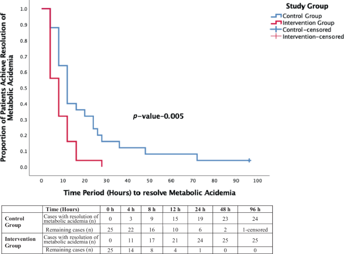
What Is a Kaplan-Meier Curve? (Background for your audience)
- The Y-axis (vertical) shows the proportion of patients who have NOT yet had the event (i.e., still unresolved acidemia). It starts at 1.0 (100% of patients unresolved) and falls toward 0 as patients achieve resolution.
- The X-axis (horizontal) shows time in hours.
- Each step downward in the curve represents one or more patients achieving the event (acidemia resolved).
- A tick mark (+) on a curve indicates a censored observation - a patient who left the study (e.g., died) before achieving the event. Their data is still used up to the point they were censored, then excluded.
Reading This Specific Graph
The Two Curves
| Control Group (Blue) | Intervention Group (Red) | |
|---|---|---|
| Treatment | WHO Ringer's Lactate only | WHO RL + bicarbonate infusion |
| Starting n | 25 | 25 |
| Curve behavior | Falls slowly, stretches to 96 hours | Falls steeply, reaches zero by ~28 hours |
Walking Through the Data Table (Step by Step)
| Time | Intervention: resolved | Intervention: remaining | Control: resolved | Control: remaining |
|---|---|---|---|---|
| 0 h | 0 | 25 | 0 | 25 |
| 4 h | 11 | 14 | 3 | 22 |
| 8 h | 17 | 8 | 9 | 16 |
| 12 h | 21 | 4 | 15 | 10 |
| 24 h | 24 | 1 | 19 | 6 |
| 48 h | 25 | 0 | 23 | 2 |
| 96 h | 25 | 0 | 24 | 1-censored |
What does this tell us?
- Intervention: 11 of 25 (44%) already resolved - nearly half the group corrected in just 4 hours
- Control: only 3 of 25 (12%) resolved - the vast majority are still acidemic
- This early divergence shows bicarbonate acts quickly
- Intervention: 17/25 (68%) resolved - the curve has crossed the 50% mark (this is the median time = 8 hours)
- Control: only 9/25 (36%) resolved - the median hasn't been reached yet
- Control: 15/25 (60%) resolved - curve finally crosses 50% (median = 12 hours)
- Intervention: 21/25 (84%) already resolved
- Intervention: All 25 patients resolved - the red curve hits zero
- Control: Still 2 patients unresolved
- One patient in the control group died before resolving acidemia
- On the graph, this appears as the small blue "+" tick at 96 hours
- KM methodology correctly excludes them from the denominator after the point of censoring, so the curve reflects the true event rate among those still being followed
The Statistical Test: Log-Rank p = 0.005
- The log-rank test compares the entire shape of both curves, not just two time points
- It asks: "Is the difference in time-to-event between the two groups larger than what we'd expect by chance?"
- p = 0.005 means there is only a 0.5% probability this difference occurred by chance
- This is highly statistically significant (well below the 5% threshold)
- The Mann-Whitney U test on the median times independently gave p = 0.0067 - consistent
The Key Takeaway in Plain Language
At every single time point measured - 4h, 8h, 12h, 24h, 48h - more children in the bicarbonate group had resolved their acidemia than in the control group. The gap opened up early and never closed. By 48 hours, every child in the bicarbonate group was corrected, while 2 in the control group were still acidemic (and one of those eventually died before correcting). The log-rank test confirms this was not a chance finding.
Important Notes for Journal Club Discussion
Explain randomization in detail
Randomization - Complete Explanation
PART 1: What Is Randomization and Why Does It Matter?
The Core Problem It Solves
- Researchers might (consciously or not) put sicker patients in the control group
- Patients who are more motivated might seek out the intervention
- Known and unknown confounding variables distort results
PART 2: Types of Randomization (General)
1. Simple Randomization
- Problem: With small samples, you can end up with unequal group sizes (e.g., 30 vs. 20 by chance)
2. Block Randomization ✅ (Used in this study)
- CCII
- CICI
- CIIC
- ICCI
- ICIC
- IICC
3. Stratified Randomization
4. Cluster Randomization
5. Adaptive Randomization
PART 3: How Randomization Was Done in THIS Study
"Block randomization with block size of 4 was done through a web-based program (http://www.randomization.com) by an individual not involved in the study. Eligible patients were randomized into control and intervention groups. Opaque sealed envelopes containing group allocation were serially numbered."
Step 1: Who generated the sequence?
Step 2: Block size = 4
Step 3: Allocation Concealment - Opaque Sealed Envelopes
- The next envelope in sequence was opened
- The allocation (Control or Intervention) inside determined the patient's group
- The envelope was opaque so the researcher could NOT see the allocation before opening it
Step 4: Was the trial blinded?
"Blinding could not be done."
- The bicarbonate solution looks different from Ringer's Lactate
- Three IV lines vs. one IV line were visually obvious
- A placebo bicarbonate infusion would be unethical without justification
- Performance bias: Clinicians may treat the intervention group differently in other ways
- Assessment bias: If the person checking blood gases knew the group, they might interpret borderline values differently (though the endpoints - pH and bicarbonate - are objective lab values, which limits this risk)
PART 4: Did Randomization Work? - Checking the Baseline Tables
| Variable | Control | Intervention | p-value | Balanced? |
|---|---|---|---|---|
| Age (months) | 4 (2,9) | 4 (3,9) | 0.73 | ✅ |
| Male sex | 68% | 48% | 0.15 | ✅ |
| Malnutrition | 72% | 72% | 1.0 | ✅ |
| Shock at admission | 16% | 20% | 1.0 | ✅ |
| Median pH | 7.1 | 7.1 | 0.77 | ✅ |
| Serum bicarbonate | 7.8 | 8.9 mEq/L | 0.55 | ✅ |
| AKI | 68% | 76% | 0.52 | ✅ |
| pSOFA score | 4 | 5 | 0.24 | ✅ |
| Platelet count | different | different | 0.02 | ⚠️ |
PART 5: Randomization Quality Assessment (CONSORT / Cochrane RoB)
Domain 1: Random Sequence Generation
- Question: Was the allocation sequence truly random?
- This study: Web-based program by an independent person ✅
- Risk of bias: LOW
Domain 2: Allocation Concealment
- Question: Was the sequence hidden until the moment of enrollment?
- This study: Opaque sealed envelopes, sequentially numbered ✅
- Risk of bias: LOW
Domain 3: Blinding of participants and personnel
- This study: Open-label - no blinding ❌
- Risk of bias: HIGH (performance bias, detection bias)
- Mitigating factor: Primary outcome (pH, serum bicarbonate) is an objective lab measurement, not subject to assessor interpretation
PART 6: The CONSORT Flow Diagram (Supplementary Fig. S1)
114 patients admitted with ADSD
        ↓
   50 eligible
        ↓
   Randomized (n=50)
    ↙           ↘
Control (n=25)   Intervention (n=25)
PART 7: Why Block Size of 4 Was the Right Choice Here
| Feature | Why it mattered in this trial |
|---|---|
| Small expected sample (~50-84 patients) | Larger blocks risk imbalance near end of trial; block size 4 kept groups even |
| Single center | No need for stratification by site |
| Short enrollment window | Block randomization ensured balance throughout, not just at the very end |
| Open-label design | Block size of 4 is small enough that prediction risk is moderate, but with open-label this was already an acknowledged limitation |
Summary for Your Presentation
This study used block randomization (block size 4) generated by an independent researcher using a web-based random number program, with allocations concealed in sequentially numbered opaque sealed envelopes. This is a methodologically sound approach that successfully balanced both known and unknown confounders - as evidenced by the comparable baseline characteristics in Tables 2 and 3. The only methodological weakness is that blinding was not possible due to the visible nature of the intervention, which is an inherent limitation of this type of fluid-based trial rather than a flaw in the randomization process itself.
Explain table 2 in detail
Table 2 - Baseline Demographic and Clinical Characteristics: Detailed Explanation
What Is the Purpose of Table 2?
Were the two groups similar before the intervention started?
Structure of the Table
- Column 1: The variable being measured
- Column 2 (Total, n=50): All 50 patients combined
- Column 3 (Control, n=25): The group that received WHO standard therapy (Ringer's Lactate only)
- Column 4 (Intervention, n=25): The group that received WHO therapy + additional bicarbonate
- Column 5 (p-value): Statistical test result comparing control vs. intervention
- Continuous variables (age, weight, scores) are reported as median (IQR) - median is the middle value, IQR = interquartile range (25th to 75th percentile). Median is used instead of mean because the data is not normally distributed (skewed by outliers)
- Categorical variables (yes/no, present/absent) are reported as n (%) - count and percentage
- Mann-Whitney U test for continuous variables (compares medians between two groups)
- Chi-square or Fisher's exact test for categorical variables (compares proportions)
- p >0.05 = no significant difference = groups are comparable ✅
Section A: Demographic Characteristics
1. Age: Median 4 months (IQR 2, 9) - p = 0.73 ✅
| Control | Intervention | |
|---|---|---|
| Median age | 4 months (IQR 2, 9) | 4 months (IQR 3, 9) |
- The median age was just 4 months in both groups - these are predominantly very young infants, not older children
- The IQR spans 2-9 months, meaning the middle 50% of patients were between 2 and 9 months old
- The study enrolled children up to 144 months (12 years), but the actual patient population skewed very young - consistent with the known epidemiology that diarrhea-related deaths are most concentrated in infants under 1 year
- p = 0.73 - no difference between groups ✅
2. Gender (Males): 29/50 (58%) overall - p = 0.15 ✅
| Control | Intervention | |
|---|---|---|
| Males | 17/25 (68%) | 12/25 (48%) |
- Overall, 58% were male - a slight male predominance, consistent with the known higher burden of diarrheal disease and dehydration in male infants in South Asia
- There is a numerical difference (68% vs. 48%) between groups, but the p-value of 0.15 tells us this is not statistically significant - it could have occurred by chance
- With only 25 patients per group, a difference of 5 patients (20%) can easily arise by chance without any real imbalance
- The groups are considered balanced for sex ✅
3. Weight-for-Age Z-score: -2.9 (-4.1, -1.6) overall - p = 0.587 ✅
| Control | Intervention | |
|---|---|---|
| WAZ score | -3.10 (-4.1, -1.75) | -2.9 (-3.8, -1.6) |
- A Z-score of -2 or below = underweight (malnutrition)
- A Z-score of -3 or below = severe underweight
- The median WAZ of -2.9 means the average patient was nearly in the severe malnutrition range
- Both groups have almost identical scores, and the p-value of 0.587 confirms balance ✅
- Malnourished children have depleted protein stores → reduced buffering capacity for acid-base changes
- They have impaired renal function → slower ability to excrete acid or regenerate bicarbonate
- They are at higher risk of mortality from metabolic acidemia
- The fact that both groups had equal malnutrition burden ensures this major risk factor did not confound the results
4. Height-for-Age Z-score: -1.4 (-2.4, -0.4) overall - p = 0.430 ✅
| Control | Intervention | |
|---|---|---|
| HAZ score | -1.25 (-2.5, 0.05) | -1.6 (-2.4, -0.90) |
- HAZ (stunting indicator) was -1.4 overall - mild stunting on average, less severe than the weight-for-age deficit
- This is consistent with chronic undernutrition in a low-middle-income country setting
- Groups are balanced (p = 0.430) ✅
5. Malnutrition (Weight-for-Age ≤ -2z): 36/50 (72%) overall - p = 0.1 ✅
| Control | Intervention | |
|---|---|---|
| Malnourished | 18/25 (72%) | 18/25 (72%) |
- 72% of all enrolled children were malnourished - a striking finding that reflects both the study setting (tertiary referral PICU in India) and the known association between malnutrition and severe diarrheal disease
- Of these 36 malnourished children, 21 (42% of total) had severe acute malnutrition (SAM) - the most extreme form
- Perfect balance: exactly 18/25 in each group (72%) ✅
- Malnutrition is one of the strongest independent risk factors for diarrheal mortality
- The fact that both groups have identical malnutrition prevalence is crucial - it means any difference in outcome is due to the bicarbonate treatment, not because one group happened to have more malnourished children
- It also means the trial results apply specifically to a malnourished population - a key point for external validity (the results may be most applicable to LMIC settings with high malnutrition burden)
Section B: Clinical Features
6. Duration of Diarrhea: Median 2 days (IQR 1, 3) - p = 0.12 ✅
| Control | Intervention | |
|---|---|---|
| Duration | 2 days (1, 3) | 1 day (1, 3) |
- Median illness duration was just 1-2 days before presentation - these children deteriorated rapidly
- This makes physiological sense: acute diarrhea causes massive, rapid bicarbonate loss through stool; within 24-48 hours, a young malnourished infant with limited reserves can develop profound sNAGMA
- p = 0.12 - not significant, groups balanced ✅
7. Fever: 19/50 (38%) overall - p = 0.77 ✅
| Control | Intervention | |
|---|---|---|
| Fever | 10/25 (40%) | 9/25 (36%) |
- 38% of patients had fever at presentation
- Fever suggests an infectious etiology (likely viral or bacterial gastroenteritis)
- Groups are balanced ✅
- Important: Children with extra-intestinal infection were excluded - so fever here is attributed to the enteric illness itself, not sepsis from another source
8. Vomiting: 44/50 (88%) overall - p = 1.0 ✅
| Control | Intervention | |
|---|---|---|
| Vomiting | 22/25 (88%) | 22/25 (88%) |
- The overwhelming majority (88%) had vomiting alongside diarrhea - this is a severely ill population
- Vomiting compounds dehydration and makes oral rehydration impossible, explaining why all these patients needed IV therapy
- Perfect balance between groups (22 in each) ✅
9. Altered Sensorium: 19/50 (38%) overall - p = 0.14 ✅
| Control | Intervention | |
|---|---|---|
| Altered sensorium | 12/25 (48%) | 7/25 (28%) |
- 38% of children had altered consciousness at presentation - a hallmark of severe metabolic acidemia and its effects on the brain
- Mechanisms: cerebral hypoperfusion from hypovolemic shock, direct neuronal suppression from severe acidosis (pH 7.09 median), and possibly electrolyte disturbances (hyponatremia in 30%, hypernatremia in 42%)
- The numerical difference (48% vs. 28%) between groups is notable, but p = 0.14 means it is not statistically significant - acceptable given the small sample size
- This is a slightly concerning imbalance numerically - the control group had more encephalopathic children at baseline, which could theoretically make them harder to treat. The authors acknowledged this as a potential limitation of the open-label small trial
10. Decreased Urine Output: 32/50 (64%) overall - p = 1.0 ✅
| Control | Intervention | |
|---|---|---|
| Decreased UO | 16/25 (64%) | 16/25 (64%) |
- 64% had oliguria at presentation - consistent with the 70% rate of AKI found on lab testing (Table 3)
- Oliguria in this context reflects:
- Severe dehydration → prerenal AKI
- Hypovolemic shock → renal hypoperfusion
- Tubular injury from prolonged acidemia and poor perfusion
- Perfect balance between groups ✅
11. pSOFA Score: Median 4 (IQR 2, 5) overall - p = 0.24 ✅
| Control | Intervention | |
|---|---|---|
| pSOFA | 4 (2, 5) | 5 (3, 5) |
- pSOFA = Pediatric Sequential Organ Failure Assessment score - measures dysfunction across 6 organ systems (respiratory, cardiovascular, neurological, hepatic, renal, coagulation)
- Score of 0 = normal; higher scores = more severe organ dysfunction
- Median pSOFA of 4-5 = moderate multi-organ dysfunction - confirming this is a critically ill population, not just moderately dehydrated children
- p = 0.24 - no significant difference ✅
12. Shock at Presentation: 9/50 (18%) overall - p = 1.0 ✅
| Control | Intervention | |
|---|---|---|
| Shock | 4/25 (16%) | 5/25 (20%) |
- 18% presented in overt shock (defined as systolic BP <5th centile for age or requiring vasoactives after >40 mL/kg fluids)
- Shock + sNAGMA = very high-risk combination; tissue hypoperfusion worsens lactic component and prevents bicarbonate regeneration
- Perfect balance (4 vs. 5), p = 1.0 ✅
13. Fluid-Refractory Shock: 6/50 (12%) overall - p = 0.38 ✅
| Control | Intervention | |
|---|---|---|
| Fluid-refractory shock | 4/25 (16%) | 2/25 (8%) |
- Fluid-refractory shock = shock that persists despite >40 mL/kg of fluid resuscitation → requires inotropes/vasopressors
- 12% overall had this most severe form of circulatory failure
- Though numerically 4 vs. 2, p = 0.38 - not significant ✅
- These are the patients who needed VIS scoring (Vasoactive Inotrope Score), and this small subgroup showed the most dramatic benefit from bicarbonate in the outcome analysis
14. Vasoactive Inotrope Score at 6 h: Median 10 (IQR 5, 10) - p = 0.48 ✅
| Control | Intervention | |
|---|---|---|
| VIS at 6h | 10 (5, 10), n=4 | 10 (10, 10), n=2 |
- This was only measured in patients who were already on inotropes (n=4 control, n=2 intervention)
- At 6 hours - before the full intervention effect - both groups had similar inotrope requirements (VIS ~10)
- This baseline equivalence is important: it confirms that by 6 hours, the inotrope need was the same in both groups. The dramatic difference in maximum VIS (34 vs. 10.5) seen later in outcomes reflects a true treatment effect, not a baseline difference
- p = 0.48 - balanced ✅
15. Coma (GCS ≤8): 1/50 (2%) overall - p = 1.0 ✅
| Control | Intervention | |
|---|---|---|
| Coma | 1/25 (4.16%) | 0/25 (0%) |
- Only 1 patient (in the control group) presented in frank coma
- Very low numbers, but both groups essentially had no comatose patients
- p = 1.0 ✅
16. Acute Kidney Injury: 35/50 (70%) overall - p = 0.52 ✅
| Control | Intervention | |
|---|---|---|
| AKI | 17/25 (68%) | 19/25 (76%) |
- 70% of enrolled children had AKI at presentation - an extraordinarily high rate that underscores the severity of illness
- AKI in this setting = prerenal/intrinsic renal injury from dehydration + hypovolemia + hyperchloremia + direct tubular toxicity from acidemia
- AKI itself impairs bicarbonate regeneration (kidneys cannot excrete H+ or reclaim HCO3-), creating a vicious cycle that makes sNAGMA even harder to correct with standard therapy alone
- This high AKI rate contextualizes why WHO therapy alone failed to correct acidemia quickly enough
- Groups balanced (p = 0.52) ✅
Overall Assessment: Did Randomization Succeed?
| Domain | Assessment |
|---|---|
| All p-values >0.05? | ✅ Yes (all 16 variables) |
| Clinically important imbalances? | ⚠️ Minor: slightly more altered sensorium in control (48% vs. 28%); slightly more fluid-refractory shock in control (16% vs. 8%) - but neither was statistically significant |
| Groups similar in severity markers (pH, SB, pSOFA, AKI)? | ✅ Yes - confirmed in Table 3 |
| Conclusion | Randomization was successful - groups are comparable at baseline |
Summary for Presentation
Table 2 presents 50 critically ill infants (median age 4 months) with the following profile: 72% malnourished, 88% vomiting, 64% oliguric, 70% with AKI, 38% with altered sensorium, and 18% in shock. Despite only 25 patients per group, block randomization successfully balanced all these characteristics. The table confirms that any difference in outcomes seen after treatment is due to the bicarbonate intervention, not pre-existing differences between groups. The population described here is a severely ill, predominantly malnourished infant cohort from a low-middle-income country tertiary center - and this defines both the internal validity (results are reliable for this population) and the external validity (results apply most directly to similar LMIC settings) of the trial.
Explain Table 3 laboratory parameters in detail
Table 3 — Baseline Laboratory Parameters: Detailed Explanation
Purpose of Table 3
How to Read the Table
- All values: Median (IQR) unless stated as n (%)
- p-value compares Control vs. Intervention
- p >0.05 = no significant difference = groups balanced ✅
- Normal reference ranges are provided below each parameter for context
SECTION A: Hematological Parameters
1. Hemoglobin (Hb): 9.9 g/dL (8.4, 11.12) — p = 0.95 ✅
| Control | Intervention | |
|---|---|---|
| Hb | 9.90 (9, 11) | 9.80 (8.2, 11.3) |
- Median Hb of 9.9 g/dL indicates mild anemia across the cohort
- In a malnourished infant population in an LMIC setting, this is expected and reflects:
- Iron deficiency (most common cause in this age group)
- Nutritional deficiencies (folate, B12)
- Chronic illness effect on erythropoiesis
- Anemia is clinically relevant here because reduced hemoglobin = reduced oxygen-carrying capacity - combined with metabolic acidosis shifting the oxygen-hemoglobin dissociation curve, tissue oxygen delivery is doubly compromised
- Perfect balance between groups (p = 0.95) ✅
2. Total Leukocyte Count (TLC): 15,990 (11,925, 20,350) cells/µL — p = 0.72 ✅
| Control | Intervention | |
|---|---|---|
| TLC | 16,000 (11,800, 19,900) | 15,800 (12,300, 21,900) |
- Median TLC of ~16,000 is at the upper limit of normal to mildly elevated, consistent with an acute infectious/inflammatory process (viral or bacterial gastroenteritis)
- Marked leukocytosis (>25,000) is not present, arguing against overwhelming bacteremia or sepsis as the primary driver - the acidemia here is predominantly from GI bicarbonate loss, not septic shock
- This supports the inclusion criteria (excluding extra-intestinal infection)
- Groups balanced (p = 0.72) ✅
3. Platelet Count: 4.47 lakh/µL (3.43, 6.51) — p = 0.02 ⚠️
| Control | Intervention | |
|---|---|---|
| Platelets | 3.65 (2.65, 5.60) lakh/µL | 5.2 (4.05, 7.8) lakh/µL |
- This is the only statistically significant baseline difference between the two groups (p = 0.02)
- The intervention group had noticeably higher platelet counts than the control group
- Both groups are within or above normal range, so neither had thrombocytopenia
- Why this likely does not matter: Platelet count is not a determinant of acid-base balance, bicarbonate levels, or acidemia resolution speed - the primary outcome. There is no biologically plausible mechanism by which higher platelets would accelerate acidemia resolution
- However, it is worth acknowledging at journal club as the one baseline imbalance - it is a product of small sample size and chance, not a flaw in randomization
Key teaching point: With only 25 patients per group, running 20+ statistical tests means you would expect at least 1 to cross the p <0.05 threshold by chance alone (Type I error). The platelet count difference is almost certainly a chance finding.
SECTION B: Blood Gas and Electrolyte Parameters
4. pH: 7.09 (6.96, 7.18) — p = 0.77 ✅
| Control | Intervention | |
|---|---|---|
| Overall median | 7.10 (7.0, 7.2) | 7.10 (7.0, 7.2) |
| pH ≤7.0 | 9 (36%) | 9 (36%) |
| pH >7.0–≤7.1 | 5 (20%) | 5 (20%) |
| pH >7.1–7.2 | 11 (44%) | 11 (44%) |
- Median pH of 7.09 - this is profound, life-threatening acidemia. Normal pH is 7.35-7.45; these children are nearly 0.3 pH units below the lower limit of normal
- Remember: pH is a logarithmic scale, so a drop from 7.40 to 7.09 represents a massive increase in hydrogen ion concentration (approximately doubled [H+])
- 36% had pH ≤7.00 - below the level at which cardiac dysfunction, arrhythmias, and vascular collapse become major risks
- The pH subgroup distribution is perfectly mirrored between the two groups (9/5/11 in both). This is the most convincing proof of successful randomization - when you see this level of balance, it cannot be attributed to anything but effective random allocation
- p = 0.77 ✅
- Up to 100 hours to resolve with WHO therapy alone (from authors' earlier 2022 study)
- Higher mortality and multi-organ failure
- Need for ventilatory support
5. Serum Bicarbonate (SB): 7.8 mEq/L (6.1, 10.5) — p = 0.55 ✅
| Control | Intervention | |
|---|---|---|
| SB | 7.8 (6.5, 9.8) | 8.9 (6.1, 11.3) |
- Median SB of 7.8 mEq/L - less than one-third of normal
- This is the direct measure of absolute bicarbonate deficiency - the core pathophysiology this trial is treating
- To put this in perspective: a normal child has ~24 mEq/L; these children had ~8 mEq/L - they have lost approximately 16 mEq/L of bicarbonate through diarrheal stool
- The IQR of 6.1–10.5 shows that the middle 50% of patients had SB between 6 and 10 - all within the "severe" NAGMA range
- Groups balanced (p = 0.55) ✅
- SB <15 was chosen as the inclusion threshold because this represents the point at which standard WHO therapy consistently fails to correct acidemia within a clinically acceptable timeframe
- SB of 15 mEq/L (not 24) was chosen as the treatment target to avoid overcorrection/alkalosis
6. Anion Gap (AG): 9.5 mEq/L (1.8–14.2) — p = 0.84 ✅
| Control | Intervention | |
|---|---|---|
| AG | 9.7 (0.6, 14) | 9.4 (2.9, 14.0) |
| AG >16, n (%) | 5 (20%) | 2 (8%) |
| Delta ratio (if AG >16) | 0.38 (0.33, 0.59) | 0.24 (0.2, 0.43) |
| Type | AG | Mechanism | Examples |
|---|---|---|---|
| NAGMA (Normal AG) | ≤16 | Bicarbonate lost directly (replaced by Cl⁻) | Diarrhea, RTA |
| HAGMA (High AG) | >16 | Unmeasured anions accumulate (acid added to body) | DKA, lactic acidosis, uraemia |
- Median AG of 9.5 mEq/L - well within the normal range, confirming this is predominantly NAGMA from diarrheal bicarbonate loss
- Children with pure NAGMA have a direct bicarbonate deficit that is logically correctable by exogenous bicarbonate replacement
- 7 patients (14%) had AG >16 (5 control, 2 intervention) - these were included only if their delta ratio was <1.0, confirming a significant NAGMA component mixed with a small HAGMA element (likely mild lactic acidosis from dehydration)
Delta ratio = (AG − 12) ÷ (24 − SB)
- <0.40 = pure NAGMA
- 0.40–0.99 = mixed NAGMA + HAGMA
- ≥1.0 = pure HAGMA (excluded from this study)
- Overall AG balance: p = 0.84 ✅
7. Lactate: 2.5 mmol/L (1.77, 4.02) — p = 0.29 ✅
| Control | Intervention | |
|---|---|---|
| Lactate | 2.5 (1.6, 3.7) | 2.6 (1.9, 5.2) |
- Median lactate of 2.5 mmol/L - mildly elevated (normal <2.0 mmol/L), consistent with mild tissue hypoperfusion from dehydration and hypovolemia
- Lactate >4.0 mmol/L would indicate severe lactic acidosis (septic shock pattern) - that is NOT the picture here
- The mild hyperlactatemia is secondary to reduced tissue perfusion from dehydration, not primary sepsis-driven lactic acidosis
- This is important because it explains why the AG is mostly normal: the lactate elevation is modest and does not push the AG above 16 in most patients
- Groups balanced (p = 0.29) ✅
SECTION C: Electrolytes
8. Serum Sodium: 144 mEq/L (133, 152) — p = 0.54 ✅
| Control | Intervention | p | |
|---|---|---|---|
| Na⁺ | 145 (136, 152) | 142 (133, 153) | 0.54 |
| Hyponatremia (<135) | 5 (20%) | 10 (40%) | 0.12 |
| Hypernatremia (>145) | 12 (48%) | 9 (36%) | 0.39 |
- Overall median of 144 mEq/L is at the upper end of normal, but the wide IQR (133–152) reveals extreme variability
- 30% had hyponatremia and 42% had hypernatremia - meaning dysnatremia was present in 72% of patients total
- This reflects the diverse fluid and electrolyte disturbances that occur with severe diarrhea
- Occurs when diarrheal losses contain proportionally more sodium than water (hypotonic diarrhea) OR when free water is given as replacement at home
- In this cohort: 15 patients (control 5, intervention 10) - numerically more in intervention but p = 0.12, not significant
- Clinically relevant because hyponatremia causes cerebral edema, seizures, and worsens sensorium - management requires modified rehydration protocols
- Occurs when water losses exceed sodium losses (hypertonic dehydration) or when inadequate free water is given
- More common in this cohort (42% vs. 30% hyponatremia)
- Hypernatremia with severe dehydration = very high-risk combination associated with seizures, intracranial hemorrhage, and cerebral edema (paradoxically, from both the hypernatremia itself and from overly rapid correction)
- 12 control vs. 9 intervention - p = 0.39, balanced ✅
- The bicarbonate solution was carefully diluted to achieve 130 mEq/L sodium - identical to Ringer's Lactate - specifically to avoid adding extra sodium to an already dysnatremic population. This was one of the most elegant design features of the study.
9. Serum Potassium: 4.8 mEq/L (3.7, 5.7) — p = 0.49 ✅
| Control | Intervention | p | |
|---|---|---|---|
| K⁺ | 4.3 (3.4, 5.7) | 4.90 (4.1, 5.6) | 0.49 |
| Hypokalemia (<3.5) | 6 (25%) | 4 (17.39%) | 0.282 |
| Hyperkalemia (>5.5) | 8 (33.3%) | 7 (30.43%) | 0.80 |
- Median K⁺ of 4.8 mEq/L is within the upper normal range at baseline
- However, the distribution is wide: 22% had hypokalemia and 30% had hyperkalemia simultaneously within the same cohort - reflecting the variable nature of potassium handling in diarrheal disease
- Large volumes of liquid stool rich in potassium cause direct GI potassium loss
- Causes: muscle weakness, cardiac arrhythmias (dangerous), ileus
- More concerning in the context of bicarbonate therapy: bicarbonate administration drives K⁺ intracellularly (alkalosis shifts K⁺ into cells), which can worsen hypokalemia - this was a key safety concern in the intervention group
- Appears paradoxical given that diarrhea causes K⁺ loss, but makes sense in the context of:
- Metabolic acidosis → H⁺ ions enter cells, K⁺ exits cells to maintain electrochemical neutrality → pseudohyperkalemia
- AKI (70% prevalence) → reduced renal K⁺ excretion
- Tissue catabolism from starvation → intracellular K⁺ release
- Hyperkalemia with severe acidosis is directly life-threatening (cardiac arrhythmias, cardiac arrest)
- Groups balanced (p = 0.49, 0.282, 0.80) ✅
10. Serum Chloride: 125 mEq/L (119, 138) — p = 0.55 ✅
| Control | Intervention | p | |
|---|---|---|---|
| Cl⁻ | 124 (120, 138) | 126 (118, 135) | 0.55 |
| Hypochloremia | 0 (0%) | 1 (4%) | 0.05 |
| Hyperchloremia | 25 (100%) | 21 (84%) | 0.055 |
- Median chloride of 125 mEq/L - dramatically above the normal upper limit of 107 mEq/L
- 92% of all patients had hyperchloremia - the control group had 100% hyperchloremia
- Bicarbonate is lost in stool
- To maintain electroneutrality, the body retains chloride to fill the gap
- Result: low bicarbonate + high chloride = hyperchloremic metabolic acidosis = NAGMA
Summary Snapshot: The "Patient Portrait" from Table 3
| Parameter | Value | What it means |
|---|---|---|
| pH | 7.09 | Profound acidemia - near incompatible with normal cardiac function |
| Serum bicarbonate | 7.8 mEq/L | One-third of normal - massive bicarbonate depletion |
| Anion gap | 9.5 mEq/L | Normal - pure NAGMA from bicarbonate loss, not acid accumulation |
| Chloride | 125 mEq/L | Hyperchloremic - confirms NAGMA mechanism |
| Lactate | 2.5 mmol/L | Mildly elevated - modest tissue hypoperfusion |
| Sodium | 144 (range 133-152) | Dysnatremia in 72% - chaotic fluid/electrolyte state |
| Potassium | 4.8 (range 3.7-5.7) | Both hypo- and hyperkalemia present - unpredictable |
| Hemoglobin | 9.9 g/dL | Mildly anaemic - reduced oxygen delivery |
| AKI | 70% | Renal impairment preventing endogenous bicarbonate regeneration |
Overall Table 3 Assessment
| Question | Answer |
|---|---|
| Were the groups biochemically similar at baseline? | Yes - 17 of 18 parameters show p >0.05 ✅ |
| Was there any meaningful imbalance? | Platelet count (p=0.02) - not clinically relevant to outcomes ⚠️ |
| Does the lab profile confirm the diagnosis of sNAGMA? | Yes - median pH 7.09, SB 7.8, AG 9.5, Cl⁻ 125 - textbook sNAGMA |
| Were exclusion criteria enforced? | Yes - low AG confirms no pure HAGMA; delta ratio confirms no pure high-AG acidosis |
| Does this population reflect the target disease? | Yes - 92% hyperchloremia, 70% AKI, profound bicarbonate depletion |
Key Presentation Point
Table 3 does two things simultaneously. First, it validates the trial design - both groups had essentially identical acid-base biochemistry before treatment, so any post-treatment difference reflects the intervention. Second, it defines the disease - a median pH of 7.09 with serum bicarbonate of 7.8 mEq/L, normal anion gap, and hyperchloremia in 92% is the biochemical signature of severe diarrheal NAGMA. Understanding this table is understanding the entire rationale for why bicarbonate - which directly replaces the depleted ion - is a physiologically logical intervention in this specific population.
Explain table 4 in detail
Table 4 — Comparison of Outcomes: Detailed Explanation
What Is Table 4?
- A. Primary Outcome — the main question the trial was designed to answer
- B. Secondary Outcomes — additional clinical endpoints
- C. Time to correct dyselectrolytemias — how quickly electrolyte abnormalities resolved
- D. New episodes of dyselectrolytemias — safety data (did the intervention cause new electrolyte problems?)
SECTION A: Primary Outcome
Time to Resolve Metabolic Acidemia (pH ≥7.30 and/or SB ≥15 mEq/L)
| Control | Intervention | p-value | |
|---|---|---|---|
| Median time (IQR) | 12 h (8, 24) | 8 h (4, 12) | 0.007 |
Breaking it down:
- Resolution was defined as achieving pH ≥7.30 AND/OR serum bicarbonate ≥15 mEq/L
- Note: this is partial correction — not full normalization to pH 7.40 or SB 24 mEq/L
- Targeting SB of 15 mEq/L (not 24) was deliberate — it avoids the risk of overcorrection and metabolic alkalosis while still lifting the patient out of the dangerous acidemia range
- Control group: median 12 hours — half the patients took more than 12 hours to reach the target
- Intervention group: median 8 hours — half the patients reached the target within 8 hours
- Difference: 4 hours faster, representing a 33% reduction in time to resolution
- Control IQR (8, 24): the middle 50% of patients took between 8 and 24 hours — a wide, unpredictable range
- Intervention IQR (4, 12): the middle 50% took between 4 and 12 hours — tighter, more predictable, and entirely earlier
- In the intervention group, 25% of patients resolved acidemia by just 4 hours — this is remarkable speed for a condition that previously took up to 100 hours to correct
- In the control group, the fastest 25% took 8 hours — double that time
SECTION B: Secondary Outcomes
B1. Time to Achieve Target Serum Bicarbonate ≥15 mEq/L
| Control | Intervention | p-value | |
|---|---|---|---|
| Median time (IQR) | 16 h (12, 30) | 8 h (4, 16) | 0.004 |
- Bicarbonate normalization took 16 hours in control vs. 8 hours in intervention — exactly half the time
- This is an even stronger difference than the primary outcome (p = 0.004 vs. 0.007)
- The IQR of control (12–30) is very wide — reflecting how unpredictable bicarbonate recovery is on WHO therapy alone
- The p-value is the smallest of all the outcome comparisons, making this the most statistically robust finding in the table
B2. Time to Achieve Target pH ≥7.30
| Control | Intervention | p-value | |
|---|---|---|---|
| Median time (IQR) | 12 h (8, 24) | 8 h (4, 12) | 0.016 |
- pH normalization followed a similar pattern — 12 hours vs. 8 hours, p = 0.016 ✅
- Note: pH correction lagged slightly behind bicarbonate correction in the control group (same median 12 h) but was faster with intervention
- This is consistent with physiology: as bicarbonate rises, the kidneys and lungs jointly normalize pH — but with very low SB, pH recovery requires the bicarbonate to reach a critical threshold first
B3. Maximum Vasoactive Inotrope Score (VIS)
| Control (n=4) | Intervention (n=2) | p-value | |
|---|---|---|---|
| Max VIS | 34 (10, 70.7) | 10.5 (10, 11) | 0.62 |
VIS = Dopamine dose + Dobutamine dose + (100 × Epinephrine dose) + (100 × Norepinephrine dose) + (10 × Milrinone dose) + (10,000 × Vasopressin dose)
- Among patients who developed fluid-refractory shock and needed inotropes:
- Control group (n=4): maximum VIS of 34 (IQR 10, 70.7) — wide range, some patients needing very high inotrope doses
- Intervention group (n=2): maximum VIS of only 10.5 (IQR 10, 11) — almost at the minimum threshold
- This is a 3-fold difference in inotrope requirements — clinically dramatic
- p = 0.62 is not statistically significant because only 4 and 2 patients are being compared — far too few for any statistical test to be meaningful
- This is a trend, not a proof — but the clinical magnitude (VIS 34 vs. 10.5) is important and hypothesis-generating for a larger trial
B4. Duration of Inotrope Support
| Control (n=5) | Intervention (n=2) | p-value | |
|---|---|---|---|
| Duration (hours) | 12 (5, 72) | 52 (20, 84) | 0.07 |
- Counterintuitively, the intervention group appears to have had longer inotrope duration — but this is misleading because:
- Only n=2 in the intervention group vs. n=5 in control — tiny numbers
- The 2 intervention patients who received inotropes may have been the most severe cases
- The VIS was much lower in intervention — they needed weaker inotropes for longer, vs. control patients needing stronger inotropes briefly (then possibly dying or deteriorating before tapering)
- p = 0.07 — not significant; numbers too small to draw conclusions
- Do not over-interpret this row
B5. Duration of Ventilation
| Control (n=3) | Intervention (n=0) | p-value | |
|---|---|---|---|
| Duration (hours) | 68 (50, 84) | 0 | — |
- 3 patients in the control group required mechanical ventilation for 50–84 hours
- Zero patients in the intervention group required ventilation
- No statistical test was possible (intervention group had no events)
- This is one of the most striking single findings in the table — an absolute difference in a devastating outcome
- Mechanically ventilating a young infant in a resource-limited PICU carries enormous risks (ventilator-associated pneumonia, barotrauma, sedation complications) and costs
- The fact that no intervention patient needed ventilation suggests that earlier acidemia resolution prevented the respiratory failure that necessitated intubation in control patients
B6. PICU Transfers
| Control | Intervention | p-value | |
|---|---|---|---|
| PICU transfers, n (%) | 5/25 (20%) | 0/25 (0%) | 0.049 |
- 20% of control patients required PICU transfer vs. 0% in the intervention group
- p = 0.049 — statistically significant (just crosses the 0.05 threshold; Fisher's exact test)
- In a resource-limited setting, PICU transfer has profound implications:
- PICU beds are scarce — a transfer may mean another patient cannot be admitted
- PICU care is dramatically more expensive and resource-intensive
- Transfer itself carries risk in critically ill infants
B7. Deaths
| Control | Intervention | p-value | |
|---|---|---|---|
| Deaths, n (%) | 2/25 (8%) | 0/25 (0%) | 0.25 |
- 2 deaths in the control group, zero in the intervention group
- p = 0.25 — not statistically significant
- With only 25 patients per group, the study was not powered (not large enough) to detect a statistically significant difference in mortality
- To detect a mortality difference of 8% vs. 0% with 80% power, you would need approximately 200+ patients per arm
- The trial was powered for the primary outcome (time to acidemia resolution), not for mortality
B8. Adverse Outcome (Composite: PICU Transfer + Deaths/LAMA)
| Control | Intervention | p-value | |
|---|---|---|---|
| Adverse outcome, n (%) | 5/25 (20%) | 0/25 (0%) | 0.049 |
- "Adverse outcome" was defined as a composite of: PICU transfer + in-hospital death + LAMA (Left Against Medical Advice — where families withdraw and leave, which the authors equate to death in terms of outcome)
- 5 patients (20%) in control vs. 0 in intervention experienced this composite
- Because PICU transfers (5) and deaths (2) overlap (both deaths occurred in the PICU), the composite equals 5 — not 7
- Fisher's exact test, p = 0.049
- Individual outcomes (deaths, PICU transfers) were too infrequent for statistical power
- Combining them into a composite endpoint increases event numbers and statistical power
- This is a standard and accepted approach in critical care trials
B9. ACAFD₅ (Acute Care Area Free Days in 5 Days)
| Control | Intervention | p-value | |
|---|---|---|---|
| ACAFD₅, median (IQR) | 1 (1, 2) | 2 (1, 2) | 0.12 |
- ACAFD₅ = 0: if patient stays in acute care for >5 days OR dies within 5 days
- ACAFD₅ = (5 − x): if patient survives and is discharged from acute care within 5 days (where x = days spent in acute care)
- Patient discharged from PER after 1 day → ACAFD₅ = 5−1 = 4
- Patient stays 3 days → ACAFD₅ = 2
- Patient dies on day 2 → ACAFD₅ = 0
- Patient stays all 5 days → ACAFD₅ = 0
- Control: median ACAFD₅ = 1 day free
- Intervention: median ACAFD₅ = 2 days free — double
- p = 0.12 — not statistically significant, but the doubling is clinically meaningful
- In a resource-constrained PER with 24,000 visits/year, freeing up acute care beds even 1 day earlier per patient has substantial system-level impact
B10. Acute Care Area Stay Among Survivors
| Control (n=23) | Intervention (n=25) | p-value | |
|---|---|---|---|
| ACA stay (hours) | 72 (48, 72) | 48 (38, 71) | 0.16 |
- Survivors in the control group spent a median of 72 hours in acute care vs. 48 hours in intervention — 24 hours less
- This is a full extra day in acute care for control survivors
- Note: this is only among survivors (n=23 control because 2 died; n=25 intervention because none died)
- p = 0.16 — not statistically significant (underpowered), but the direction and magnitude are clinically relevant
B11. Hospital Stay Among Survivors
| Control (n=23) | Intervention (n=25) | p-value | |
|---|---|---|---|
| Hospital stay (hours) | 72 (48, 96) | 48 (46, 70) | 0.076 |
- Total hospital stay: control median 72 hours vs. intervention 48 hours — 24 hours shorter
- p = 0.076 — just misses significance (likely because the study is underpowered for this endpoint)
- A reduction of 24 hours in hospital stay, if confirmed in a larger trial, would have enormous cost and resource implications at scale
SECTION C: Time to Correct Dyselectrolytemias
C1. Hypernatremia
| Control (n=12) | Intervention (n=9) | p-value | |
|---|---|---|---|
| Time to correct (hours) | 14 (4, 27) | 24 (6, 50) | 0.39 |
- Numerically, hypernatremia appeared to take longer to correct in the intervention group (24 vs. 14 hours), but p = 0.39 — not significant
- This is reassuring: the bicarbonate infusion, despite containing sodium, did not worsen or prolong hypernatremia
- The careful sodium-matched dilution protocol (130 mEq/L in both groups) prevented additional sodium loading
C2. Hyponatremia
| Control (n=4) | Intervention (n=10) | p-value | |
|---|---|---|---|
| Time to correct (hours) | 8 (8, 11) | 6 (4, 8) | 0.10 |
- Hyponatremia actually trended toward faster correction in the intervention group (6 vs. 8 hours), but numbers are too small
- p = 0.10 — not significant ✅
C3. Hypokalemia
| Control (n=7) | Intervention (n=4) | p-value | |
|---|---|---|---|
| Time to correct (hours) | 8 (4, 12) | 12 (9, 12) | 0.21 |
- Numerically, hypokalemia took slightly longer to correct in intervention (12 vs. 8 hours)
- This is biologically plausible — bicarbonate drives K⁺ intracellularly, potentially prolonging hypokalemia slightly
- However, p = 0.21 — not significant, and the difference is small ✅
C4. Hyperkalemia
| Control (n=8) | Intervention (n=7) | p-value | |
|---|---|---|---|
| Time to correct (hours) | 8 (4, 8) | 8 (4, 8) | 0.648 |
- Perfect equivalence — both groups corrected hyperkalemia in 8 hours
- Bicarbonate drives K⁺ into cells → would be expected to help correct hyperkalemia faster, but this did not translate to a measurable difference here
- p = 0.648 — completely balanced ✅
SECTION D: New Episodes of Dyselectrolytemias (Safety Data)
D1. New Hypernatremia
| Control | Intervention | p-value | |
|---|---|---|---|
| n (%) | 5 (20%) | 4 (16%) | 0.50 |
- No increase in hypernatremia with bicarbonate ✅
- This directly refutes the commonest concern: that sodium bicarbonate will cause hypernatremia from sodium loading
- The isonatremic dilution protocol (130 mEq/L) was the key design feature that prevented this
D2. New Hyponatremia
| Control | Intervention | p-value | |
|---|---|---|---|
| n (%) | 1 (4%) | 2 (8%) | 0.50 |
- Negligible new hyponatremia in both groups — p = 0.50 ✅
D3. New Hyperkalemia
| Control | Intervention | p-value | |
|---|---|---|---|
| n (%) | 0 (0%) | 0 (0%) | — |
- Zero new hyperkalemia in either group ✅
- Bicarbonate was expected to drive K⁺ into cells and potentially unmask hypokalemia, not cause hyperkalemia — this is consistent
D4. New Hypokalemia ← Most Watched Safety Parameter
| Control | Intervention | p-value | |
|---|---|---|---|
| n (%) | 16 (64%) | 16 (64%) | 1.0 |
- This is the critical safety finding: 64% of both groups developed hypokalemia — identical rates
- The bicarbonate infusion did NOT increase hypokalemia risk beyond the baseline risk of the disease itself
- This is the strongest safety evidence in the paper, because hypokalemia was the most theoretically probable adverse effect
- The disease itself causes K⁺ loss through diarrheal stool
- Rehydration with any fluid dilutes plasma K⁺
- Correction of acidemia (whether by bicarbonate or RL) shifts K⁺ intracellularly
- These mechanisms are universal in this disease — adding bicarbonate did not make it worse
Additional Safety Findings (Mentioned in Text, Not in Table)
- Hypocalcemia: None in either group ✅
- Deterioration in sensorium: None in intervention group ✅ (directly refutes concern about paradoxical CSF acidosis or cerebral edema)
- Metabolic alkalosis overshoot: None documented ✅
- Need for renal replacement therapy in intervention: None ✅
Master Summary Table
| Outcome | Control | Intervention | p-value | Significant? |
|---|---|---|---|---|
| Time to resolve acidemia | 12 h | 8 h | 0.007 | ✅ YES |
| Time to target SB ≥15 | 16 h | 8 h | 0.004 | ✅ YES |
| Time to target pH ≥7.30 | 12 h | 8 h | 0.016 | ✅ YES |
| PICU transfers | 20% | 0% | 0.049 | ✅ YES |
| Adverse outcome composite | 20% | 0% | 0.049 | ✅ YES |
| Deaths | 8% | 0% | 0.25 | ❌ (underpowered) |
| ACAFD₅ | 1 day | 2 days | 0.12 | ❌ (trend) |
| Hospital stay | 72 h | 48 h | 0.076 | ❌ (trend) |
| Max VIS | 34 | 10.5 | 0.62 | ❌ (n too small) |
| Ventilation needed | 3 patients | 0 patients | — | No test possible |
| New hypokalemia | 64% | 64% | 1.0 | ✅ SAFE |
| New hypernatremia | 20% | 16% | 0.50 | ✅ SAFE |
| New hypocalcemia | 0% | 0% | — | ✅ SAFE |
| Worsening sensorium | 0% | 0% | — | ✅ SAFE |
The Core Message of Table 4 for Your Presentation
Table 4 shows that adding calculated-dose bicarbonate to WHO rehydration therapy produced three statistically significant benefits: faster resolution of acidemia (primary outcome, p=0.007), faster bicarbonate normalization (p=0.004), and fewer adverse outcomes including PICU transfers and deaths (p=0.049). Clinically meaningful trends — halving of hospital stay, doubling of free days, elimination of ventilator use, threefold reduction in inotrope requirements — consistently favored the intervention but did not reach significance due to small sample size. Critically, the intervention caused no additional electrolyte disturbances of any kind. The safety profile was identical to standard care. This combination of significant efficacy on the primary outcome, a significant composite safety-and-clinical outcome, and a clean adverse-effect profile makes a compelling case for a larger multicentric confirmatory trial.
What is single center study
Single-Center Study — Complete Explanation
Definition
In the Context of This Article
- The single center: Advanced Pediatrics Center, PGIMER, Chandigarh, India
- A 1,950-bed multispecialty tertiary teaching hospital
- Pediatric Emergency Room: ~24,000 visits/year, admits ~12,000/year
- PICU: 15 beds, admits ~950 patients/year, ventilates ~400/year
- All 50 patients were enrolled, treated, and followed up at this one institution
- One team managed the entire trial — the authors themselves
Why Single-Center Studies Are Done
| Reason | Explanation |
|---|---|
| Feasibility | Easier to coordinate — one ethics committee, one protocol, one team |
| Control | Uniform application of inclusion/exclusion criteria |
| Consistency | Same lab analyzers, same nursing care, same monitoring standards |
| Speed | Quicker to start — no need to train multiple sites |
| Cost | Much cheaper than coordinating across hospitals |
| Pilot purpose | Often done first to test whether a larger multicentric trial is justified |
Advantages of a Single-Center Study
1. Standardized Protocol Application
2. Uniform Laboratory Methods
3. Tight Quality Control
4. No Inter-Site Heterogeneity
5. Rapid Execution
Limitations of a Single-Center Study — Why This Matters for Your Journal Club
1. External Validity / Generalizability ← Most Important Limitation
- More severely ill than average (selection bias at the population level)
- From a specific geographic region (North India)
- Predominantly from lower socioeconomic groups
- Subject to this hospital's specific pathogens, antibiotic resistance patterns, and nutritional epidemiology
- Community hospitals with less severe patient populations
- Hospitals in different countries with different diarrheal pathogens
- Settings with different nutritional profiles or different access to IV therapy
- Private hospitals or high-income country settings
2. Sample Size Limitation
- Had to cut recruitment from 18 months to 12 months (COVID-19)
- Ended with only 50 patients — too few to detect differences in mortality (which needs 200+ patients)
- Subgroup analyses (e.g., SB <5 vs. >10) had only 3–6 patients — not interpretable statistically
3. Assessment Bias Risk
- Clinicians may (unconsciously) monitor the intervention group more closely
- Decisions about PICU transfer (part of the primary composite outcome) may be influenced by knowing the group
- The authors acknowledge: "PICU bed may not be available at a time when children actually need it" — at one center, bed availability is finite and inconsistent
4. Local Expertise Effect ("Center Effect")
- Calculating and preparing the bicarbonate dilution correctly
- Managing fluid-refractory shock in infants
- Recognizing sNAGMA early and enrolling appropriately
5. Cannot Adjust for Unmeasured Confounders Across Settings
Single-Center vs. Multicenter: Head-to-Head Comparison
| Feature | Single-Center (This Study) | Multicenter (Future Trial Recommended) |
|---|---|---|
| Sample size | Small (n=50) | Large (hundreds to thousands) |
| Protocol consistency | High ✅ | Variable ⚠️ |
| Generalizability | Limited ⚠️ | High ✅ |
| Power for rare outcomes (mortality) | Low ⚠️ | High ✅ |
| Cost and logistics | Low ✅ | High ⚠️ |
| Time to complete | Fast ✅ | Slow ⚠️ |
| Detection of subgroup effects | Underpowered ⚠️ | Possible ✅ |
| Risk of center-specific bias | Higher ⚠️ | Diluted across sites ✅ |
| Appropriate for | Pilot/proof-of-concept ✅ | Definitive guideline-changing evidence ✅ |
Where Does a Single-Center RCT Sit in the Evidence Hierarchy?
Systematic Review / Meta-analysis         ← Highest
        ↑
Multicenter RCT (large, blinded)
        ↑
Single-center RCT ← THIS STUDY           ← Here
        ↑
Prospective cohort study
        ↑
Retrospective cohort / Case-control
        ↑
Case series / Case reports
        ↑
Expert opinion                            ← Lowest
How the Authors Address This Limitation
"The study provides encouraging and clinically relevant data to inform a large multi-centric trial in LMICs with high burden of diarrheal diseases. Blinding and stratification based on SB levels are advisable for future multi-centric trials."
- Proof of concept — does bicarbonate help at all? Answer: yes
- Safety signal — does it cause harm? Answer: no
- Effect size estimation — how big is the benefit? Answer: 33% reduction in time, 20% vs. 0% adverse outcomes
- Justification for investment in a larger multicentric trial
Summary for Your Presentation
A single-center study means all 50 patients were enrolled and treated at one hospital — PGIMER Chandigarh. This gives the study high internal consistency (same team, same lab, same protocol) but limits external validity (can we apply these results everywhere?). It is the appropriate design for a first trial of this intervention — generating the proof-of-concept and safety data needed before a larger multicentric trial. The results are compelling, but the next step — stratified, blinded, multicentric RCT across multiple LMICs — is needed before these findings can change international guidelines.
How is P value calculated
How Is the P-Value Calculated? — Complete Explanation
What Is a P-Value? (Start Here)
"If there were truly no difference between the two treatments, what is the probability of seeing a difference this large (or larger) just by chance?"
- Small p-value (e.g., p = 0.007): This difference would be very unlikely by chance alone → the difference is probably real → statistically significant
- Large p-value (e.g., p = 0.72): This difference could easily occur by chance → we cannot conclude a real difference exists → not statistically significant
The Null Hypothesis — The Foundation
H₀: "There is NO difference between the control and intervention groups"
The General Process of P-Value Calculation
Step 1: Choose the Right Statistical Test
Step 2: Calculate the Test Statistic
Step 3: Find Where That Number Falls on a Known Distribution
Step 4: Read Off the P-Value
The Three Statistical Tests Used in This Article
"Mann-Whitney U test and Chi-square test (or Fisher's exact test) were used for intergroup comparisons. Time taken to resolve metabolic acidemia was compared by Kaplan-Meier curve after censoring deaths."
TEST 1: Mann-Whitney U Test
When was it used?
Why not a regular t-test?
How It Works — Step by Step
- Control group (n=25): times in hours e.g., 8, 8, 12, 12, 24...
- Intervention group (n=25): times in hours e.g., 4, 4, 8, 8, 12...
| Rank | Time (h) | Group |
|---|---|---|
| 1 | 4 | Intervention |
| 2 | 4 | Intervention |
| 3 | 8 | Control |
| 4 | 8 | Intervention |
| ... | ... | ... |
| 50 | 96 | Control |
- Sum of ranks for Intervention group = R₁
- Sum of ranks for Control group = R₂
U₁ = n₁ × n₂ + [n₁(n₁+1)/2] − R₁ U₂ = n₁ × n₂ − U₁
Z = (U − n₁n₂/2) ÷ √[n₁n₂(n₁+n₂+1)/12]
TEST 2: Chi-Square Test (χ²)
When was it used?
The Core Idea
How It Works — Step by Step
- Control: 5 transferred, 20 not transferred
- Intervention: 0 transferred, 25 not transferred
- Total: 5 transferred out of 50 (10% overall)
| PICU Transfer | No Transfer | Total | |
|---|---|---|---|
| Control | 5 | 20 | 25 |
| Intervention | 0 | 25 | 25 |
| Total | 5 | 45 | 50 |
Expected = (Row total × Column total) ÷ Grand total
| PICU Transfer | No Transfer | |
|---|---|---|
| Control (expected) | (25×5)/50 = 2.5 | (25×45)/50 = 22.5 |
| Intervention (expected) | (25×5)/50 = 2.5 | (25×45)/50 = 22.5 |
χ² = Σ [(Observed − Expected)² ÷ Expected]
- Control, PICU: (5−2.5)²/2.5 = 6.25/2.5 = 2.5
- Control, No PICU: (20−22.5)²/22.5 = 6.25/22.5 = 0.278
- Intervention, PICU: (0−2.5)²/2.5 = 6.25/2.5 = 2.5
- Intervention, No PICU: (25−22.5)²/22.5 = 6.25/22.5 = 0.278
TEST 3: Fisher's Exact Test
When is it used instead of Chi-square?
How It Works
p = (R₁! × R₂! × C₁! × C₂!) ÷ (N! × Π aᵢⱼ!)
TEST 4: Log-Rank Test (for the Kaplan-Meier Curve)
When was it used?
How It Works
- How many events were observed in each group
- How many events were expected if there were no difference (based on the proportion at risk in each group at that moment)
Expected events in group 1 = (n₁ at risk / total at risk) × total events at time t
χ²_logrank = [Σ(O₁ − E₁)]² ÷ Var(O₁ − E₁)
Visualizing What a P-Value Actually Is
                    NULL HYPOTHESIS DISTRIBUTION
                    (what we'd expect by chance)

                         ████
                       ████████
                     ████████████
                   ████████████████
                 ████████████████████
               ████████████████████████
             ████████████████████████████
─────────────────────────────────────────────────
                                     ↑        ↑
                              p=0.05 cutoff   Your test statistic
                              (5% of area)    (only 0.7% area beyond here)
                                              → p = 0.007
Common Misconceptions — Important for Journal Club
| Misconception | Reality |
|---|---|
| p < 0.05 means the result is "true" | It means the result is unlikely to be due to chance — it could still be a false positive (1 in 20 by definition) |
| p = 0.049 is more meaningful than p = 0.051 | This arbitrary cutoff is a convention — a result just above 0.05 is not "proven negative" |
| A large p-value means no effect exists | It means there is insufficient evidence to detect an effect — often because the sample is too small |
| p-value tells you the size of the effect | No — it only tells you statistical significance. Effect size (e.g., 4-hour difference, 20% vs 0%) is separate |
| p < 0.05 is always clinically meaningful | Not necessarily — a tiny, clinically irrelevant difference can be statistically significant with a large enough sample |
How the P-Values in This Paper Were Calculated — Quick Reference
| Outcome | Test Used | Why That Test |
|---|---|---|
| Age, weight-z, Hb, pH, SB (median data) | Mann-Whitney U | Non-normal distribution, comparing medians |
| Fever, vomiting, AKI (yes/no proportions) | Chi-square | Adequate expected cell counts |
| PICU transfers, deaths (small counts) | Fisher's exact | Expected cells <5 |
| Time-to-event (KM curves) | Log-rank | Survival/time-to-event data with censoring |
| All tests | Two-tailed at α=0.05 | Standard threshold for medical research |
Summary for Your Presentation
A p-value is the probability of seeing your results by chance if the null hypothesis were true. In this paper, three different tests were used depending on the data type: Mann-Whitney U for comparing medians (non-normal continuous data), Chi-square/Fisher's exact for comparing proportions (categorical yes/no data), and the log-rank test for comparing time-to-event curves. All tests follow the same logical chain: calculate a test statistic from your data → locate it on a known mathematical distribution → read off the tail probability (p-value). A p-value of 0.007 for the primary outcome means there is only a 0.7% probability that the observed 4-hour difference in acidemia resolution arose by chance alone — strong evidence that bicarbonate genuinely accelerated recovery.
WHO criteria of dehydration
WHO criteria dehydration assessment children diarrhea classification 2005
https://medicalguidelines.msf.org/en/viewport/CG/english/deh…
WHO Criteria for Dehydration in Children — Complete Explanation
Why This Matters for the Article
The Core Concept: How Dehydration Is Assessed
WHO Three-Category Classification
CATEGORY 1: No Dehydration (< 5% fluid loss)
| Clinical Sign | Finding |
|---|---|
| Mental status | Well, alert |
| Eyes | Normal |
| Thirst / drinking | Drinks normally, not thirsty |
| Skin pinch | Goes back quickly (< 2 seconds) |
- Continue breastfeeding
- Give extra ORS (oral rehydration solution) after each loose stool
- ORS volume: 50–100 mL after each stool for children < 2 years; 100–200 mL for older children
- Return if condition worsens, cannot drink, develops fever, blood in stool
CATEGORY 2: Some Dehydration (5–10% fluid loss)
| Clinical Sign | Finding |
|---|---|
| Mental status | Restless or irritable |
| Eyes | Sunken |
| Thirst / drinking | Thirsty, drinks eagerly |
| Skin pinch | Goes back slowly (2–3 seconds) |
- Give ORS: 75 mL/kg over 4 hours in a supervised setting
- Reassess every 1–2 hours
- If vomiting > 2 times, give by nasogastric tube
- After 4 hours, reassess and reclassify
- If improving → continue Plan B or switch to Plan A
- If worsening → upgrade to Plan C
| Age | Weight | ORS over 4 hours |
|---|---|---|
| < 4 months | < 5 kg | 200–400 mL |
| 4–11 months | 5–7.9 kg | 400–600 mL |
| 12–23 months | 8–10.9 kg | 600–800 mL |
| 2–4 years | 11–15.9 kg | 800–1200 mL |
| 5–14 years | 16–29.9 kg | 1200–2200 mL |
CATEGORY 3: Severe Dehydration (> 10% fluid loss) ← The Category in This Study
| Clinical Sign | Finding |
|---|---|
| Mental status | Lethargy or unconsciousness |
| Eyes | Sunken (deeply) |
| Thirst / drinking | Unable to drink or drinks poorly |
| Skin pinch | Goes back very slowly (≥ 2 seconds) |
WHO Treatment Plan C (IV Rehydration) — This Is What the Study Used
For Children ≥ 1 Year (majority of this study — age >1 yr or >10 kg):
| IV Fluid | Volume | Rate |
|---|---|---|
| Ringer's Lactate (preferred) | 100 mL/kg total | 30 mL/kg in first 30 minutes, then 70 mL/kg over next 2.5 hours |
For Infants < 1 Year (age <1 yr or <10 kg):
| IV Fluid | Volume | Rate |
|---|---|---|
| Ringer's Lactate | 100 mL/kg total | 30 mL/kg in first 1 hour, then 70 mL/kg over next 5 hours |
Reassessment every 30 minutes:
- If radial pulse is still very weak → repeat the 30 mL/kg bolus
- If improving → complete the infusion
- If shock signs persist after full Plan C → evaluate for septic shock, switch to sepsis protocol
The Four Key Clinical Signs Explained in Detail
1. Mental Status / Level of Consciousness
| Severity | Finding | Underlying Mechanism |
|---|---|---|
| No dehydration | Alert, playful | Normal cerebral perfusion |
| Some dehydration | Restless, irritable | Early hypoperfusion; child uncomfortable |
| Severe dehydration | Lethargic / unconscious | Severe hypovolemia → reduced cerebral blood flow + metabolic acidemia suppressing CNS |
2. Eyes
| Severity | Finding |
|---|---|
| No dehydration | Normal |
| Some dehydration | Sunken |
| Severe dehydration | Deeply sunken |
3. Thirst / Ability to Drink
| Severity | Finding |
|---|---|
| No dehydration | Drinks normally, not thirsty |
| Some dehydration | Thirsty, drinks eagerly when offered |
| Severe dehydration | Unable to drink or drinks poorly |
- Severely altered sensorium → cannot coordinate swallowing
- Extreme weakness/lethargy
- Shock → reduced gastrointestinal motility
- This also explains why ALL enrolled patients in the article needed IV therapy — they could not take adequate oral fluids
4. Skin Pinch (Skin Turgor Test) — Most Objective Sign
| Result | Classification |
|---|---|
| Returns immediately (<1 second) | No dehydration |
| Returns slowly (goes back over 1–2 seconds) | Some dehydration |
| Returns very slowly (≥ 2 seconds, "tenting") | Severe dehydration |
- Malnutrition: Malnourished children have reduced subcutaneous fat → skin always has poor turgor even without dehydration. Skin pinch overestimates dehydration in SAM. In this study (72% malnourished), this sign required careful interpretation.
- Hypernatremic dehydration: Skin retains turgor better (feels "doughy") because hypertonicity keeps fluid in the interstitium → skin pinch may underestimate dehydration severity. In this study, 42% had hypernatremia — meaning skin turgor was relatively preserved despite severe dehydration in many patients.
- Obese children: Excess subcutaneous fat gives falsely normal turgor.
Summary Comparison Table (WHO 2005)
| Feature | No Dehydration | Some Dehydration | Severe Dehydration |
|---|---|---|---|
| % fluid loss | <5% | 5–10% | >10% |
| Deficit (infants) | <50 mL/kg | 50–100 mL/kg | >100 mL/kg |
| Mental status | Alert | Restless/irritable | Lethargic/unconscious |
| Eyes | Normal | Sunken | Deeply sunken |
| Drinking | Normal | Thirsty, drinks eagerly | Cannot drink |
| Skin pinch | Returns quickly | Returns slowly | Returns very slowly (≥2 sec) |
| Signs required | None from above | ≥ 2 of the above | ≥ 2 of the above |
| Treatment | Plan A (home ORS) | Plan B (supervised ORS, 75 mL/kg/4h) | Plan C (IV RL urgently) |
Additional Clinical Signs (Not in the 4-Sign Rule but Clinically Assessed)
| Sign | Relevance |
|---|---|
| Capillary refill > 2 sec | Suggests poor peripheral perfusion; supports severe dehydration |
| Sunken fontanelle (infants) | Reflects reduced intracranial CSF volume — a reliable sign in infants <18 months |
| Absent tears | Loss of lacrimal secretion with hypovolemia |
| Dry mucous membranes | Dry mouth and tongue; less reliable in mouth-breathing children |
| Tachycardia | Compensatory; heart rate rises before BP falls |
| Hypotension | Late sign — indicates decompensated shock; systolic BP <5th centile for age |
| Reduced urine output | 64% had oliguria in this study |
| Weak/absent radial pulse | Indicates impending circulatory collapse |
The Shock Threshold Within Severe Dehydration
- 18% had shock at presentation (systolic BP <5th centile for age OR requiring vasoactives after >40 mL/kg)
- 12% had fluid-refractory shock (persisting despite full fluid resuscitation)
Why Ringer's Lactate and Not Normal Saline?
| Fluid | Na⁺ | K⁺ | Cl⁻ | Bicarbonate equivalent | Osmolarity |
|---|---|---|---|---|---|
| Ringer's Lactate | 130 | 4 | 109 | 28 (as lactate) | 273 mOsm/L |
| Normal Saline (0.9%) | 154 | 0 | 154 | None | 308 mOsm/L |
- Lactate is metabolized by the liver → converted to bicarbonate → helps correct acidemia
- Lower chloride → does not worsen hyperchloremia
- More physiologically balanced (closer to plasma composition)
- Cochrane 2023 review confirmed: RL gives higher final pH (+0.06) and bicarbonate (+2.44 mEq/L) vs. normal saline in children with diarrhea and severe dehydration
Key Teaching Point for Your Presentation
The WHO dehydration criteria are a clinical bedside tool based on 4 key signs: mental status, eyes, ability to drink, and skin turgor — with ≥2 signs required for each level. Severe dehydration (≥2 severe signs) mandates immediate IV rehydration with Ringer's Lactate at 100 mL/kg (Plan C). In this study, all 50 enrolled children met severe dehydration criteria AND had sNAGMA on top of it — a combination that WHO Plan C alone was insufficient to manage, providing the entire rationale for the bicarbonate trial.