Levels of health care

Reading File

Finding Sources

Searching the Web

levels of health care primary secondary tertiary quaternary

Reading File

Here is a complete overview of the Levels of Health Care, drawn directly from Park's Textbook of Preventive and Social Medicine:

Levels of Health Care

Health services are organized at three levels, each supported by a higher level to which patients can be referred. These levels represent different types of care involving varying degrees of complexity.

1. Primary Health Care (PHC)

The first level of contact between the individual, family, community, and the national health system.
Provides "essential" (basic) health care - the most fundamental and broadest level.
Closest to the people - a majority of prevailing health problems can be satisfactorily dealt with and resolved here.
In the Indian context, primary health care is provided by:
- Primary Health Centres (PHCs) and their sub-centres
- Multipurpose health workers, ANMs, ASHAs, Anganwadi workers, village health guides, trained dais
Village health teams also bridge the cultural and communication gap between rural populations and the organised health sector.
Since India adopted "Health for All" by 2000 AD, the PHC system has been restructured and strengthened.

2. Secondary Health Care

The next higher level - also called the intermediate health care level.
Deals with more complex problems that cannot be managed at the primary level.
Comprises essentially curative services.
Serves as the first referral level in the health system.
In India, provided by:
- District Hospitals
- Community Health Centres (CHCs)
Patients are referred upward from the primary level when needed.

3. Tertiary Health Care

The most specialised level, requiring specific facilities and highly specialised health workers.
Offers super-specialist care for complex, rare, or difficult conditions.
Provided by regional/central level institutions, e.g.:
- Medical College Hospitals
- All India Institutes (e.g., AIIMS)
- Regional Hospitals, Specialised Hospitals, Apex Institutions
Functions include:
- Providing highly specialised clinical care
- Planning and managerial functions
- Teaching of specialised staff
- Supporting and complementing actions carried out at the primary level

The Referral System

A fundamental requirement linking all three levels is a sound referral system. It must be a two-way exchange - patients referred upward for specialist care, and returned to the referring provider for follow-up. This ensures:

Continuity of care
Consumer confidence in the health system

For many developing countries, including India, this referral linkage remains an area requiring significant strengthening.

Summary Table

Feature	Primary	Secondary	Tertiary
Level of contact	First (direct)	Second (referral)	Third (referral)
Complexity	Basic/essential	Intermediate	Super-specialist
Focus	Preventive + curative	Mainly curative	Highly specialised curative
Indian facilities	PHC, sub-centres	District hospitals, CHCs	Medical colleges, AIIMS, Apex institutions
Population served	Broadest	District level	Regional/national

Source: Park's Textbook of Preventive and Social Medicine (the standard reference for community medicine in India)

Note: Some frameworks also describe a Quaternary level (an extension of tertiary care involving experimental medicine, highly advanced diagnostic/surgical procedures, and research - found mainly in high-income country systems), though the classical public health model used in India focuses on three levels.

Sensitivity and specificity

Finding Sources

Searching the Web

sensitivity specificity positive predictive value negative predictive value diagnostic tests

Reading File

Loading Image

Finding Sources

Here is a thorough breakdown of Sensitivity and Specificity drawn from Henry's Clinical Diagnosis and Management by Laboratory Methods, Tietz Textbook of Laboratory Medicine, and Creasy & Resnik's Maternal-Fetal Medicine.

Sensitivity and Specificity

The 2 × 2 Contingency Table

All measures of diagnostic accuracy are derived from this fundamental table:

	Disease Present	Disease Absent
Test Positive	True Positive (TP)	False Positive (FP)
Test Negative	False Negative (FN)	True Negative (TN)

Definitions

Sensitivity

The ability of a test to detect disease when it is truly present.
The proportion of persons with disease in whom the test is positive.
Also called the True Positive Rate (TPR).

Sensitivity = TP / (TP + FN)

Inverse: (1 - Sensitivity) = False Negative Rate (FNR)
A test with 90% sensitivity will correctly identify 90 out of 100 diseased patients, and miss 10 (false negatives).
A highly sensitive test is good for ruling OUT disease - a negative result on a highly sensitive test makes disease unlikely. Mnemonic: SnNout (Sensitive test, Negative result, rules Out disease).

Specificity

The ability of a test to detect the absence of disease when it is truly absent.
The proportion of persons without disease in whom the test is negative.
Also called the True Negative Rate (TNR).

Specificity = TN / (TN + FP)

Inverse: (1 - Specificity) = False Positive Rate (FPR)
A test with 90% specificity will correctly identify 90 out of 100 disease-free patients; 10 will test falsely positive.
A highly specific test is good for ruling IN disease - a positive result on a highly specific test strongly indicates disease. Mnemonic: SpPin (Specific test, Positive result, rules In disease).

Key Distinction

Property	Based on	Used to
Sensitivity	Diseased population	Rule OUT disease
Specificity	Non-diseased population	Rule IN disease
Both are independent of disease prevalence

Worked Example (Cardiac Marker Study)

	Disease (AMI)	No Disease	Total
Test Positive	196 (TP)	20 (FP)	216
Test Negative	4 (FN)	180 (TN)	184
Total	200	200	400

Sensitivity = 196 / (196 + 4) = 98%
Specificity = 180 / (180 + 20) = 90%
PPV = 196 / (196 + 20) = 91%
NPV = 180 / (180 + 4) = 98%

(From Henry's Clinical Diagnosis and Management by Laboratory Methods)

Predictive Values

Unlike sensitivity and specificity, predictive values depend on disease prevalence.

Positive Predictive Value (PPV)

The probability that a patient with a positive test truly has the disease.

PPV = TP / (TP + FP)

Negative Predictive Value (NPV)

The probability that a patient with a negative test truly does not have the disease.

NPV = TN / (TN + FN)

Effect of Prevalence

Prevalence	PPV	NPV
Increases	Increases	Decreases
Decreases	Decreases	Increases

This is why the same test used in a high-risk clinic (high prevalence) will have a better PPV than when used for general population screening (low prevalence).

The Cutoff Effect: Sensitivity vs. Specificity Trade-off

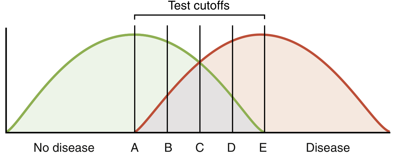
Effects of varying the test cutoff on overlapping disease and no-disease populations

Figure: Effects of varying the test cutoff on overlapping populations. Green = no disease; Red = disease. The overlap zone is where false results occur.

When the cutoff is lowered (shifted left, from C → B → A):
- Sensitivity increases (more diseased patients captured)
- Specificity decreases (more non-diseased patients also test positive)
When the cutoff is raised (shifted right, from C → D → E):
- Specificity increases (fewer false positives)
- Sensitivity decreases (more diseased patients are missed)

This inverse relationship is the fundamental trade-off in diagnostic testing.

When to Prioritize Sensitivity vs. Specificity

Clinical Goal	Choose	Reason
Screening for serious disease	High Sensitivity	Minimize false negatives; don't miss cases
Confirming diagnosis before toxic/costly treatment	High Specificity	Minimize false positives; avoid unnecessary harm
Ruling out disease	High Sensitivity	SnNout
Ruling in disease	High Specificity	SpPin

Example: PSA screening for prostate cancer uses a low threshold (high sensitivity) - many men without cancer test positive and undergo biopsy, but no true cancers are missed. A confirmatory test like GC/MS for drugs of abuse uses high specificity to avoid false accusations.

Diagnostic Accuracy

Diagnostic Accuracy = (TP + TN) / (TP + TN + FP + FN)

This is the overall proportion of correctly classified subjects. However, it can be misleading when disease prevalence is very low or very high, which is why sensitivity, specificity, PPV, and NPV together give a more complete picture.

Summary Mnemonics

Mnemonic	Meaning
SnNout	Sensitive test + Negative result = rules out disease
SpPin	Specific test + Positive result = rules in disease

Sources: Henry's Clinical Diagnosis and Management by Laboratory Methods; Tietz Textbook of Laboratory Medicine, 7th Ed.; Creasy & Resnik's Maternal-Fetal Medicine

Make this pdf

Reading File

Running Command

ls /home/daytona/workspace/

Writing File

~/sensitivity_specificity.py

from reportlab.lib.pagesizes import A4
from reportlab.lib import colors
from reportlab.lib.styles import getSampleStyleSheet, ParagraphStyle
from reportlab.lib.units import cm
from reportlab.platypus import (
    SimpleDocTemplate, Paragraph, Spacer, Table, TableStyle,
    HRFlowable, KeepTogether
)
from reportlab.lib.enums import TA_CENTER, TA_LEFT, TA_JUSTIFY
from reportlab.platypus import Image as RLImage
import urllib.request
import os

OUTPUT = "/home/daytona/workspace/Sensitivity_and_Specificity.pdf"

# Download the cutoff diagram
img_url = "https://cdn.orris.care/cdss_images/8e0506db858047f18f43cc365f485002710895064ee8a2883dec8c3cf601000a.png"
img_path = "/home/daytona/workspace/cutoff_diagram.png"
urllib.request.urlretrieve(img_url, img_path)

doc = SimpleDocTemplate(
    OUTPUT,
    pagesize=A4,
    rightMargin=2*cm,
    leftMargin=2*cm,
    topMargin=2.2*cm,
    bottomMargin=2*cm,
)

W, H = A4
body_width = W - 4*cm

# ── Colour palette ──────────────────────────────────────────────
NAVY    = colors.HexColor("#1A3A5C")
TEAL    = colors.HexColor("#0D7C7C")
LIGHT   = colors.HexColor("#E8F4F4")
ACCENT  = colors.HexColor("#C0392B")
GRAY    = colors.HexColor("#F4F6F8")
MID     = colors.HexColor("#5D7A8A")
WHITE   = colors.white
BLACK   = colors.black

styles = getSampleStyleSheet()

def S(name, **kw):
    return ParagraphStyle(name, **kw)

title_style = S("Title2",
    fontName="Helvetica-Bold", fontSize=22,
    textColor=WHITE, alignment=TA_CENTER,
    spaceAfter=6, leading=28)

sub_style = S("Sub",
    fontName="Helvetica", fontSize=11,
    textColor=colors.HexColor("#AECBCB"), alignment=TA_CENTER,
    spaceAfter=4)

h1 = S("H1",
    fontName="Helvetica-Bold", fontSize=13,
    textColor=NAVY, spaceBefore=14, spaceAfter=4, leading=18)

h2 = S("H2",
    fontName="Helvetica-Bold", fontSize=11,
    textColor=TEAL, spaceBefore=10, spaceAfter=3, leading=15)

body = S("Body2",
    fontName="Helvetica", fontSize=10,
    textColor=BLACK, spaceAfter=5, leading=15, alignment=TA_JUSTIFY)

formula = S("Formula",
    fontName="Helvetica-Bold", fontSize=11,
    textColor=ACCENT, spaceAfter=4, leading=16, alignment=TA_CENTER)

caption = S("Caption",
    fontName="Helvetica-Oblique", fontSize=8.5,
    textColor=MID, alignment=TA_CENTER, spaceAfter=6)

bullet = S("Bullet",
    fontName="Helvetica", fontSize=10,
    textColor=BLACK, spaceAfter=3, leading=14,
    leftIndent=18, bulletIndent=6)

mnemonic = S("Mnemonic",
    fontName="Helvetica-Bold", fontSize=11,
    textColor=WHITE, alignment=TA_CENTER, leading=16)

source_style = S("Source",
    fontName="Helvetica-Oblique", fontSize=7.5,
    textColor=MID, alignment=TA_CENTER, spaceAfter=2)

# ── Helper: coloured section header box ─────────────────────────
def section_header(text, bg=NAVY):
    data = [[Paragraph(text, ParagraphStyle("SH",
        fontName="Helvetica-Bold", fontSize=13,
        textColor=WHITE, alignment=TA_LEFT, leading=17))]]
    t = Table(data, colWidths=[body_width])
    t.setStyle(TableStyle([
        ("BACKGROUND", (0,0), (-1,-1), bg),
        ("LEFTPADDING",  (0,0), (-1,-1), 10),
        ("RIGHTPADDING", (0,0), (-1,-1), 10),
        ("TOPPADDING",   (0,0), (-1,-1), 6),
        ("BOTTOMPADDING",(0,0), (-1,-1), 6),
        ("ROUNDEDCORNERS", [4]),
    ]))
    return t

# ── Helper: formula box ─────────────────────────────────────────
def formula_box(text):
    data = [[Paragraph(text, ParagraphStyle("FB",
        fontName="Helvetica-Bold", fontSize=12,
        textColor=ACCENT, alignment=TA_CENTER, leading=17))]]
    t = Table(data, colWidths=[body_width*0.7])
    t.setStyle(TableStyle([
        ("BACKGROUND", (0,0), (-1,-1), colors.HexColor("#FDF2F1")),
        ("BOX",        (0,0), (-1,-1), 1.2, ACCENT),
        ("LEFTPADDING",(0,0), (-1,-1), 14),
        ("RIGHTPADDING",(0,0),(-1,-1), 14),
        ("TOPPADDING",  (0,0),(-1,-1), 7),
        ("BOTTOMPADDING",(0,0),(-1,-1), 7),
        ("ALIGN",      (0,0), (-1,-1), "CENTER"),
    ]))
    return t

def centered(t):
    wrapper = Table([[t]], colWidths=[body_width])
    wrapper.setStyle(TableStyle([
        ("ALIGN",(0,0),(-1,-1),"CENTER"),
        ("LEFTPADDING",(0,0),(-1,-1),0),
        ("RIGHTPADDING",(0,0),(-1,-1),0),
        ("TOPPADDING",(0,0),(-1,-1),0),
        ("BOTTOMPADDING",(0,0),(-1,-1),0),
    ]))
    return wrapper

# ════════════════════════════════════════════════════════════════
story = []

# ── TITLE BANNER ────────────────────────────────────────────────
banner_data = [[
    Paragraph("Sensitivity &amp; Specificity", title_style),
    ],[
    Paragraph("Diagnostic Test Performance | Epidemiology &amp; Biostatistics", sub_style),
]]
banner = Table(banner_data, colWidths=[body_width])
banner.setStyle(TableStyle([
    ("BACKGROUND", (0,0), (-1,-1), NAVY),
    ("LEFTPADDING",  (0,0), (-1,-1), 16),
    ("RIGHTPADDING", (0,0), (-1,-1), 16),
    ("TOPPADDING",   (0,0), (-1,-1), 18),
    ("BOTTOMPADDING",(0,0), (-1,-1), 18),
    ("ROUNDEDCORNERS", [6]),
]))
story.append(banner)
story.append(Spacer(1, 0.4*cm))

# ── 2x2 TABLE SECTION ───────────────────────────────────────────
story.append(section_header("The 2 × 2 Contingency Table"))
story.append(Spacer(1, 0.25*cm))

two_by_two = [
    ["", "Disease Present", "Disease Absent"],
    ["Test Positive", "True Positive (TP)", "False Positive (FP)"],
    ["Test Negative", "False Negative (FN)", "True Negative (TN)"],
]
cell_style = ParagraphStyle("cell", fontName="Helvetica", fontSize=10, alignment=TA_CENTER, leading=14)
bold_cell  = ParagraphStyle("bcell", fontName="Helvetica-Bold", fontSize=10, alignment=TA_CENTER, leading=14, textColor=WHITE)
normal_cell= ParagraphStyle("ncell", fontName="Helvetica", fontSize=10, alignment=TA_CENTER, leading=14, textColor=BLACK)

tw = body_width
col1, col2, col3 = tw*0.25, tw*0.375, tw*0.375
t2 = Table([
    ["", Paragraph("Disease Present", bold_cell), Paragraph("Disease Absent", bold_cell)],
    [Paragraph("Test Positive", bold_cell), Paragraph("True Positive (TP)", normal_cell), Paragraph("False Positive (FP)", normal_cell)],
    [Paragraph("Test Negative", bold_cell), Paragraph("False Negative (FN)", normal_cell), Paragraph("True Negative (TN)", normal_cell)],
], colWidths=[col1, col2, col3])
t2.setStyle(TableStyle([
    ("BACKGROUND", (0,0), (0,2), NAVY),
    ("BACKGROUND", (1,0), (2,0), TEAL),
    ("BACKGROUND", (0,0), (0,0), colors.HexColor("#0A2540")),
    ("BACKGROUND", (1,1), (1,1), colors.HexColor("#D5EAD5")),
    ("BACKGROUND", (2,1), (2,1), colors.HexColor("#FAD9D5")),
    ("BACKGROUND", (1,2), (1,2), colors.HexColor("#FAD9D5")),
    ("BACKGROUND", (2,2), (2,2), colors.HexColor("#D5EAD5")),
    ("GRID",       (0,0), (-1,-1), 0.5, colors.HexColor("#AAAAAA")),
    ("ALIGN",      (0,0), (-1,-1), "CENTER"),
    ("VALIGN",     (0,0), (-1,-1), "MIDDLE"),
    ("TOPPADDING", (0,0), (-1,-1), 8),
    ("BOTTOMPADDING",(0,0),(-1,-1), 8),
]))
story.append(t2)
story.append(Spacer(1, 0.3*cm))

# ── DEFINITIONS ─────────────────────────────────────────────────
story.append(section_header("Core Definitions", bg=TEAL))
story.append(Spacer(1, 0.25*cm))

# Sensitivity & Specificity side by side
def def_box(title, color, formula_text, lines, note):
    items = [Paragraph(f"<b><font color='white'>{title}</font></b>",
                ParagraphStyle("dbt", fontName="Helvetica-Bold", fontSize=11,
                               textColor=WHITE, alignment=TA_CENTER, leading=15))]
    for line in lines:
        items.append(Paragraph(f"• {line}",
            ParagraphStyle("dbb", fontName="Helvetica", fontSize=9.5,
                           textColor=BLACK, leading=13, leftIndent=6)))
    items.append(Spacer(1, 4))
    items.append(Paragraph(formula_text,
        ParagraphStyle("dbf", fontName="Helvetica-Bold", fontSize=10.5,
                       textColor=ACCENT, alignment=TA_CENTER, leading=14)))
    items.append(Spacer(1, 4))
    items.append(Paragraph(f"<i>{note}</i>",
        ParagraphStyle("dbn", fontName="Helvetica-Oblique", fontSize=9,
                       textColor=MID, alignment=TA_CENTER, leading=12)))

    inner = Table([[item] for item in items],
                  colWidths=[body_width*0.46])
    inner.setStyle(TableStyle([
        ("BACKGROUND", (0,0), (0,0), color),
        ("BACKGROUND", (0,1), (-1,-1), GRAY),
        ("TOPPADDING",    (0,0), (-1,-1), 6),
        ("BOTTOMPADDING", (0,0), (-1,-1), 6),
        ("LEFTPADDING",   (0,0), (-1,-1), 10),
        ("RIGHTPADDING",  (0,0), (-1,-1), 10),
        ("BOX",           (0,0), (-1,-1), 0.8, color),
    ]))
    return inner

sens_box = def_box(
    "SENSITIVITY (True Positive Rate)",
    TEAL,
    "Sensitivity = TP / (TP + FN)",
    [
        "Ability to detect disease when present",
        "Proportion of diseased patients who test positive",
        "1 − Sensitivity = False Negative Rate",
        "90% sensitivity → misses 10 of 100 cases",
    ],
    "High sensitivity → Rule OUT disease (SnNout)"
)
spec_box = def_box(
    "SPECIFICITY (True Negative Rate)",
    NAVY,
    "Specificity = TN / (TN + FP)",
    [
        "Ability to detect absence of disease",
        "Proportion of non-diseased who test negative",
        "1 − Specificity = False Positive Rate",
        "90% specificity → 10 false positives per 100",
    ],
    "High specificity → Rule IN disease (SpPin)"
)

side_by_side = Table([[sens_box, Spacer(0.2*cm, 1), spec_box]],
                     colWidths=[body_width*0.47, 0.06*body_width, body_width*0.47])
side_by_side.setStyle(TableStyle([
    ("ALIGN",  (0,0), (-1,-1), "CENTER"),
    ("VALIGN", (0,0), (-1,-1), "TOP"),
    ("LEFTPADDING",  (0,0), (-1,-1), 0),
    ("RIGHTPADDING", (0,0), (-1,-1), 0),
    ("TOPPADDING",   (0,0), (-1,-1), 0),
    ("BOTTOMPADDING",(0,0), (-1,-1), 0),
]))
story.append(side_by_side)
story.append(Spacer(1, 0.4*cm))

# ── MNEMONICS ───────────────────────────────────────────────────
mnem_data = [
    [Paragraph("<b>SnNout</b>", ParagraphStyle("mn1", fontName="Helvetica-Bold", fontSize=12, textColor=WHITE, alignment=TA_CENTER)),
     Paragraph("<b>SpPin</b>",  ParagraphStyle("mn2", fontName="Helvetica-Bold", fontSize=12, textColor=WHITE, alignment=TA_CENTER))],
    [Paragraph("Sensitive test + Negative result<br/>→ Rules OUT disease",
               ParagraphStyle("md1", fontName="Helvetica", fontSize=9.5, textColor=BLACK, alignment=TA_CENTER, leading=14)),
     Paragraph("Specific test + Positive result<br/>→ Rules IN disease",
               ParagraphStyle("md2", fontName="Helvetica", fontSize=9.5, textColor=BLACK, alignment=TA_CENTER, leading=14))],
]
mnem_table = Table(mnem_data, colWidths=[body_width*0.48, body_width*0.48],
                   spaceBefore=0, spaceAfter=0)
mnem_table.setStyle(TableStyle([
    ("BACKGROUND", (0,0), (0,0), TEAL),
    ("BACKGROUND", (1,0), (1,0), NAVY),
    ("BACKGROUND", (0,1), (0,1), colors.HexColor("#E0F4F4")),
    ("BACKGROUND", (1,1), (1,1), colors.HexColor("#E0EAF4")),
    ("ALIGN",      (0,0), (-1,-1), "CENTER"),
    ("VALIGN",     (0,0), (-1,-1), "MIDDLE"),
    ("TOPPADDING", (0,0), (-1,-1), 7),
    ("BOTTOMPADDING",(0,0),(-1,-1), 7),
    ("BOX",        (0,0), (0,-1), 0.8, TEAL),
    ("BOX",        (1,0), (1,-1), 0.8, NAVY),
    ("GRID",       (0,0), (-1,-1), 0.5, colors.HexColor("#CCCCCC")),
]))

mnem_wrapper = Table([[mnem_table]], colWidths=[body_width])
mnem_wrapper.setStyle(TableStyle([
    ("ALIGN",(0,0),(-1,-1),"CENTER"),
    ("LEFTPADDING",(0,0),(-1,-1),0),
    ("RIGHTPADDING",(0,0),(-1,-1),0),
    ("TOPPADDING",(0,0),(-1,-1),0),
    ("BOTTOMPADDING",(0,0),(-1,-1),0),
    ("COLWIDTH", (0,0), (-1,-1), body_width*0.96),
]))
story.append(mnem_wrapper)
story.append(Spacer(1, 0.4*cm))

# ── PREDICTIVE VALUES ───────────────────────────────────────────
story.append(section_header("Predictive Values (Prevalence-Dependent)", bg=colors.HexColor("#4A235A")))
story.append(Spacer(1, 0.25*cm))

pv_text = [
    ("PPV — Positive Predictive Value",
     "PPV = TP / (TP + FP)",
     "Probability that a POSITIVE test result truly means disease is present."),
    ("NPV — Negative Predictive Value",
     "NPV = TN / (TN + FN)",
     "Probability that a NEGATIVE test result truly means disease is absent."),
]
for title, form, desc in pv_text:
    story.append(Paragraph(f"<b>{title}</b>", h2))
    story.append(Paragraph(desc, body))
    fbox = formula_box(form)
    story.append(centered(fbox))
    story.append(Spacer(1, 0.15*cm))

story.append(Spacer(1, 0.1*cm))
story.append(Paragraph("<b>Effect of Prevalence on Predictive Values</b>", h2))

prev_data = [
    ["Prevalence", "PPV", "NPV"],
    ["Increases ↑", "Increases ↑", "Decreases ↓"],
    ["Decreases ↓", "Decreases ↓", "Increases ↑"],
]
pv_table = Table(prev_data, colWidths=[body_width/3]*3)
pv_table.setStyle(TableStyle([
    ("BACKGROUND", (0,0), (-1,0), colors.HexColor("#4A235A")),
    ("TEXTCOLOR",  (0,0), (-1,0), WHITE),
    ("FONTNAME",   (0,0), (-1,0), "Helvetica-Bold"),
    ("BACKGROUND", (0,1), (-1,1), colors.HexColor("#F0E8F5")),
    ("BACKGROUND", (0,2), (-1,2), colors.HexColor("#FAF0FF")),
    ("ALIGN",      (0,0), (-1,-1), "CENTER"),
    ("FONTSIZE",   (0,0), (-1,-1), 10),
    ("GRID",       (0,0), (-1,-1), 0.5, colors.HexColor("#AAAAAA")),
    ("TOPPADDING", (0,0), (-1,-1), 7),
    ("BOTTOMPADDING",(0,0),(-1,-1), 7),
]))
story.append(pv_table)
story.append(Spacer(1, 0.4*cm))

# ── CUTOFF DIAGRAM ──────────────────────────────────────────────
story.append(section_header("The Cutoff Effect: Sensitivity-Specificity Trade-off", bg=colors.HexColor("#7D3C00")))
story.append(Spacer(1, 0.3*cm))

img = RLImage(img_path, width=body_width*0.85, height=body_width*0.35)
img_wrapper = Table([[img]], colWidths=[body_width])
img_wrapper.setStyle(TableStyle([
    ("ALIGN",(0,0),(-1,-1),"CENTER"),
    ("TOPPADDING",(0,0),(-1,-1),0),
    ("BOTTOMPADDING",(0,0),(-1,-1),0),
]))
story.append(img_wrapper)
story.append(Paragraph(
    "Figure: Effects of varying the test cutoff. Green = no disease distribution; "
    "Red = disease distribution. Overlap zone = false results.",
    caption))

cutoff_data = [
    ["Cutoff Direction", "Sensitivity", "Specificity", "FP Rate", "FN Rate"],
    ["Lowered (Left: C→B→A)", "↑ Increases", "↓ Decreases", "↑ More FPs", "↓ Fewer FNs"],
    ["Raised (Right: C→D→E)", "↓ Decreases", "↑ Increases", "↓ Fewer FPs", "↑ More FNs"],
]
ct = Table(cutoff_data, colWidths=[body_width*0.28, body_width*0.18, body_width*0.18, body_width*0.18, body_width*0.18])
ct.setStyle(TableStyle([
    ("BACKGROUND", (0,0), (-1,0), colors.HexColor("#7D3C00")),
    ("TEXTCOLOR",  (0,0), (-1,0), WHITE),
    ("FONTNAME",   (0,0), (-1,0), "Helvetica-Bold"),
    ("BACKGROUND", (0,1), (-1,1), colors.HexColor("#FFF3E0")),
    ("BACKGROUND", (0,2), (-1,2), colors.HexColor("#FFF8EE")),
    ("ALIGN",      (0,0), (-1,-1), "CENTER"),
    ("FONTSIZE",   (0,0), (-1,-1), 9),
    ("GRID",       (0,0), (-1,-1), 0.5, colors.HexColor("#AAAAAA")),
    ("TOPPADDING", (0,0), (-1,-1), 7),
    ("BOTTOMPADDING",(0,0),(-1,-1), 7),
]))
story.append(ct)
story.append(Spacer(1, 0.4*cm))

# ── WORKED EXAMPLE ──────────────────────────────────────────────
story.append(section_header("Worked Example — Cardiac Marker (AMI)", bg=colors.HexColor("#145A32")))
story.append(Spacer(1, 0.25*cm))
story.append(Paragraph(
    "In an evaluation study of a hypothetical cardiac marker, 200 patients with acute myocardial infarction (AMI) "
    "and 200 healthy subjects are recruited (prevalence = 50%). The 2 × 2 truth table:", body))

ex_data = [
    ["", "Disease (AMI) n=200", "No Disease n=200", "Total"],
    ["Test Positive", "196 (TP)", "20 (FP)", "216"],
    ["Test Negative", "4 (FN)", "180 (TN)", "184"],
    ["Total", "200", "200", "400"],
]
ex_table = Table(ex_data, colWidths=[body_width*0.28, body_width*0.24, body_width*0.24, body_width*0.24])
ex_table.setStyle(TableStyle([
    ("BACKGROUND", (0,0), (-1,0), colors.HexColor("#145A32")),
    ("TEXTCOLOR",  (0,0), (-1,0), WHITE),
    ("FONTNAME",   (0,0), (-1,0), "Helvetica-Bold"),
    ("BACKGROUND", (0,0), (0,-1), colors.HexColor("#1E8449")),
    ("TEXTCOLOR",  (0,1), (0,-1), WHITE),
    ("BACKGROUND", (1,1), (1,1), colors.HexColor("#D5F5E3")),
    ("BACKGROUND", (2,1), (2,1), colors.HexColor("#FADBD8")),
    ("BACKGROUND", (1,2), (1,2), colors.HexColor("#FADBD8")),
    ("BACKGROUND", (2,2), (2,2), colors.HexColor("#D5F5E3")),
    ("BACKGROUND", (0,3), (-1,3), GRAY),
    ("FONTNAME",   (0,3), (-1,3), "Helvetica-Bold"),
    ("ALIGN",      (0,0), (-1,-1), "CENTER"),
    ("FONTSIZE",   (0,0), (-1,-1), 10),
    ("GRID",       (0,0), (-1,-1), 0.5, colors.HexColor("#AAAAAA")),
    ("TOPPADDING", (0,0), (-1,-1), 7),
    ("BOTTOMPADDING",(0,0),(-1,-1), 7),
]))
story.append(ex_table)
story.append(Spacer(1, 0.2*cm))

results_data = [
    ["Measure", "Formula", "Result"],
    ["Sensitivity",  "196 / (196 + 4)",   "98%"],
    ["Specificity",  "180 / (180 + 20)",  "90%"],
    ["PPV",          "196 / (196 + 20)",  "91%"],
    ["NPV",          "180 / (180 + 4)",   "98%"],
]
res_table = Table(results_data, colWidths=[body_width*0.28, body_width*0.42, body_width*0.30])
res_table.setStyle(TableStyle([
    ("BACKGROUND", (0,0), (-1,0), colors.HexColor("#145A32")),
    ("TEXTCOLOR",  (0,0), (-1,0), WHITE),
    ("FONTNAME",   (0,0), (-1,0), "Helvetica-Bold"),
    ("BACKGROUND", (0,1), (-1,-1), colors.HexColor("#EAFAF1")),
    ("FONTNAME",   (2,1), (2,-1), "Helvetica-Bold"),
    ("TEXTCOLOR",  (2,1), (2,-1), colors.HexColor("#145A32")),
    ("ALIGN",      (0,0), (-1,-1), "CENTER"),
    ("FONTSIZE",   (0,0), (-1,-1), 10),
    ("GRID",       (0,0), (-1,-1), 0.5, colors.HexColor("#AAAAAA")),
    ("TOPPADDING", (0,0), (-1,-1), 7),
    ("BOTTOMPADDING",(0,0),(-1,-1), 7),
    ("ROWBACKGROUNDS", (0,1), (-1,-1), [colors.HexColor("#EAFAF1"), colors.HexColor("#D5F5E3")]),
]))
story.append(res_table)
story.append(Spacer(1, 0.4*cm))

# ── CLINICAL GUIDE ──────────────────────────────────────────────
story.append(section_header("When to Use High Sensitivity vs. High Specificity", bg=MID))
story.append(Spacer(1, 0.2*cm))

cg_data = [
    ["Clinical Goal", "Priority", "Reason", "Example"],
    ["Screen for serious disease", "High\nSensitivity", "Don't miss cases\n(minimize FN)", "PSA for prostate cancer"],
    ["Confirm before toxic therapy", "High\nSpecificity", "Avoid false positives\n(minimize FP)", "Confirmatory HIV test"],
    ["Rule OUT disease", "High\nSensitivity", "SnNout", "D-dimer for PE"],
    ["Rule IN disease", "High\nSpecificity", "SpPin", "Troponin for AMI"],
]
cg_table = Table(cg_data, colWidths=[body_width*0.30, body_width*0.18, body_width*0.27, body_width*0.25])
cg_table.setStyle(TableStyle([
    ("BACKGROUND", (0,0), (-1,0), MID),
    ("TEXTCOLOR",  (0,0), (-1,0), WHITE),
    ("FONTNAME",   (0,0), (-1,0), "Helvetica-Bold"),
    ("ROWBACKGROUNDS", (0,1), (-1,-1),
     [colors.HexColor("#EBF5FB"), colors.HexColor("#F4F6F7")]),
    ("ALIGN",      (0,0), (-1,-1), "CENTER"),
    ("VALIGN",     (0,0), (-1,-1), "MIDDLE"),
    ("FONTSIZE",   (0,0), (-1,-1), 9),
    ("GRID",       (0,0), (-1,-1), 0.5, colors.HexColor("#AAAAAA")),
    ("TOPPADDING", (0,0), (-1,-1), 7),
    ("BOTTOMPADDING",(0,0),(-1,-1), 7),
]))
story.append(cg_table)
story.append(Spacer(1, 0.4*cm))

# ── DIAGNOSTIC ACCURACY ─────────────────────────────────────────
story.append(section_header("Overall Diagnostic Accuracy", bg=colors.HexColor("#2C3E50")))
story.append(Spacer(1, 0.2*cm))
story.append(Paragraph(
    "The overall proportion of correctly classified subjects:", body))
story.append(centered(formula_box("Diagnostic Accuracy = (TP + TN) / (TP + TN + FP + FN)")))
story.append(Spacer(1, 0.15*cm))
story.append(Paragraph(
    "Note: Overall accuracy can be misleading when disease prevalence is very low or very high. "
    "Using sensitivity, specificity, PPV, and NPV together gives a more complete and balanced picture "
    "of a test's performance.", body))
story.append(Spacer(1, 0.4*cm))

# ── SOURCE ──────────────────────────────────────────────────────
HRFlowable_line = HRFlowable(width="100%", thickness=0.5, color=MID)
story.append(HRFlowable_line)
story.append(Spacer(1, 0.1*cm))
story.append(Paragraph(
    "Sources: Henry's Clinical Diagnosis and Management by Laboratory Methods | "
    "Tietz Textbook of Laboratory Medicine, 7th Ed. | "
    "Creasy &amp; Resnik's Maternal-Fetal Medicine",
    source_style))

# ── BUILD ────────────────────────────────────────────────────────
doc.build(story)
print(f"PDF created: {OUTPUT}")

Running Command

cd /home/daytona/workspace && python sensitivity_specificity.py

Your PDF is ready! Here's what's included:

Sensitivity and Specificity

PDF Document · PDF

The document covers:

2 × 2 Contingency Table - colour-coded TP/FP/FN/TN cells
Sensitivity & Specificity - side-by-side definition boxes with formulas
SnNout / SpPin mnemonics - highlighted in teal and navy
Predictive Values (PPV & NPV) - with the effect of prevalence table
Cutoff Effect diagram - the actual textbook figure showing overlapping distributions
Worked Example - the AMI cardiac marker study with all four calculated values
Clinical Guide - when to prioritise sensitivity vs. specificity with real examples (PSA, troponin, D-dimer)
Overall Diagnostic Accuracy formula
Source citations at the bottom

This is a shared conversation. Sign in to Orris to start your own chat.