
Ppt of 25 slides on cardiac physiology for md residents
cardiac action potential conduction system heart
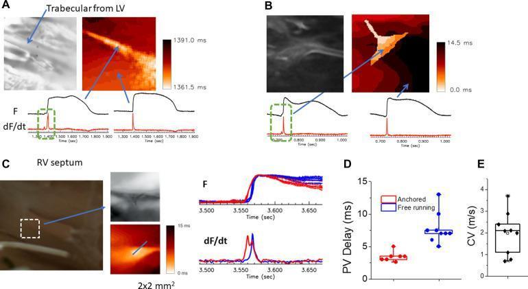
Educational panel illustrating cardiac electrophysiology and optical mapping of the Purkinje-ventricular junction (PVJ) in rabbit heart models. The figure is divided into five sections (A-E). Panels A, B, and C present side-by-side anatomical grayscale/brightfield images, color-coded activation maps, and corresponding action potential traces (F) with their first derivatives (dF/dt). These panels demonstrate conduction in the trabecular muscle of the left ventricle (A), free-running Purkinje fibers (B), and the right ventricular (RV) septum involving papillary muscle (C). A key educational feature is the visualization of 'step-delays' in the dF/dt traces—highlighted by green dotted boxes—showing dual upstrokes that represent the temporal separation between Purkinje fiber activation and ventricular muscle activation. Panel D provides a comparative dot plot of Purkinje-ventricular (PV) delay in milliseconds, distinguishing between 'anchored' (shorter delay) and 'free-running' (longer delay) fibers. Panel E is a box-and-whisker plot displaying the conduction velocity (CV) along Purkinje fibers, measured in meters per second (m/s). This resource illustrates how the specialized conduction system coordinates rapid, sequential electrical activation within the ventricular myocardium.
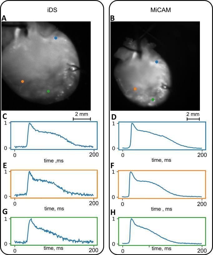
This Comparison Chart illustrates cardiac optical mapping data obtained from two different camera systems: the iDS (left column) and MiCAM (right column). Panels A and B display still frames of a Langendorff-perfused mouse heart, stained with a voltage-sensitive dye (Di-4-ANEPPS). Three color-coded pixels (blue, orange, and green) are marked on the ventricular surface of each heart image, indicating specific regions of interest. Panels C through H present the corresponding action potential (AP) waveforms recorded from these marked locations. The x-axis represents time in milliseconds (0–200 ms) and the y-axis shows normalized signal amplitude. The AP waveforms demonstrate characteristic cardiac electrophysiological phases, including rapid depolarization and subsequent repolarization. Visually, the iDS system images (A) appear brighter with a clearer anatomical outline but show higher high-frequency noise in the raw AP traces (C, E, G). In contrast, the state-of-the-art MiCAM system (B) produces traces with a higher signal-to-noise ratio (D, F, H), resulting in smoother AP curves. This comparison is used in cardiovascular research to validate the efficacy of lower-cost imaging systems for measuring cardiac activation sequences and action potential duration (APD).
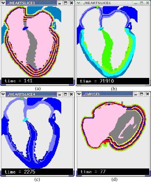
This composite image presents four panels (a–d) of computerized cardiac simulations focusing on stratified heart wall models and electrophysiological properties. Panel (a) shows a 2-D stratified heart model with multi-colored concentric layers representing the endocardium-to-epicardium transition in the ventricular walls. Panel (b) illustrates a 2-D simulation of epicardium-to-endocardium repolarization, with a color gradient (green to dark blue) mapped to transmembrane potential across the myocardium. Panel (c) highlights two areas of myocardial ischemia, visualized through variations in blue and cyan shades. Panel (d) displays a cross-sectional view of a 3-D stratified model, further demonstrating the arc-shaped fiber orientation and wall layering. The models utilize cellular automata to represent different cardiac tissues, including the sinoatrial node (SAN), atrioventricular node (AVN), and the conduction system (bundle branches and Purkinje fibers). These simulations are designed for medical education and research into arrhythmia generation, ischemia effects, and the electrical heterogeneity of the heart walls, particularly the simulation of M cells and transmural action potential duration gradients.
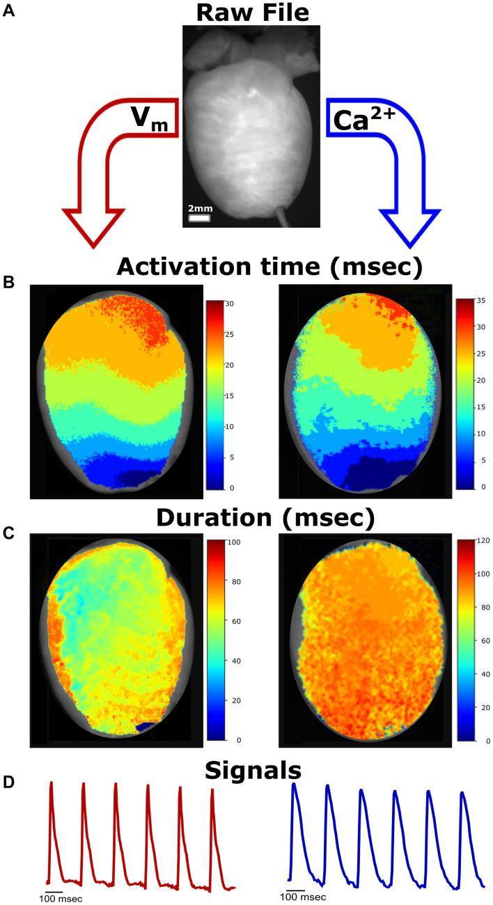
This composite educational graphic illustrates the workflow for cardiac optical mapping, specifically focusing on the simultaneous analysis of transmembrane voltage (Vm) and intracellular calcium (Ca2+) in a mammalian heart model. Panel A shows the raw grayscale image of a Langendorff-perfused heart. Panel B presents activation time maps in milliseconds (msec) for both Vm and Ca2+. These pseudocolor maps demonstrate the propagation of electrical and calcium signals from the apex (blue, indicating earlier activation) toward the base (red, indicating later activation), reflecting the coordinated cardiac conduction sequence. Panel C displays duration maps for the action potential and calcium transients. The Vm duration map (left) utilizes a scale up to 100 msec, while the Ca2+ duration map (right) extends to 120 msec, highlighting the characteristically longer duration of calcium transients. Panel D provides representative temporal signal traces, showing the morphology of repetitive action potentials and calcium transients. This figure serves as a diagnostic tool for evaluating excitation-contraction coupling and regional heterogeneity in cardiac electrophysiology.
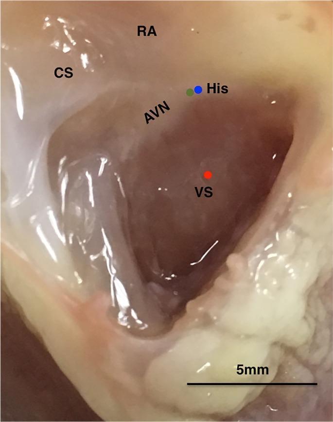
An anatomical clinical photograph of an experimental rabbit heart preparation, used for cardiac electrophysiology research. The image displays the right atrial endocardium and basal ventricular septum after the removal of the right atrium (RA) to expose the cardiac conduction system. Key anatomical landmarks are labeled: the coronary sinus (CS), the atrioventricular node (AVN), the His bundle (His), and the ventricular septum (VS). Specific experimental recording sites are marked with colored dots: a green dot indicates the position of a bipolar electrode on the His bundle; a blue dot represents the site of a glass microelectrode impalement into the His bundle; and a red dot marks the microelectrode recording site on the endocardium of the ventricular septum. A 5 mm scale bar is provided at the bottom right for spatial reference. The photograph demonstrates the anatomical relationships necessary for simultaneous intracellular action potential recording from the specialized conduction system and working myocardium.
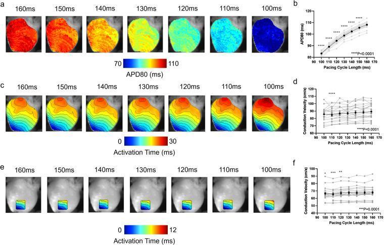
This composite educational image illustrates the restitution dynamics of the heart using optical mapping in a guinea pig model. The content is divided into six panels (a-f) focusing on electrophysiological parameters. Panel (a) presents high-resolution false-color maps showing the action potential duration at 80% repolarization (APD80). As the pacing cycle length (PCL) decreases from 160ms to 100ms, a visible transition from red (longer APD80, ~110ms) to blue (shorter APD80, ~70ms) occurs, a trend quantified in the corresponding line graph (b). Panels (c) and (e) display activation maps where color and isochronal lines represent electrical impulse travel time. Panel (c) shows whole-heart activation, while (e) restricts the analysis to a specific apical region. These maps demonstrate changes in activation patterns and timing as PCL shortens. Panels (d) and (f) provide statistical grouped data for conduction velocity (CV) as a function of PCL, showing a significant decrease in CV with shorter cycle lengths. This figure is critical for understanding cardiac electrophysiology, rate-dependent remodeling, and arrhythmogenesis markers like APD restitution and conduction slowing.
Frank-Starling curve cardiac output preload ventricular function
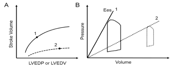
Summary : This figure compares cardiac function under two conditions using two types of plots: (A) the Frank-Starling relationship between stroke volume and left ventricular filling, and (B) pressure-volume loops with end-systolic elastance (Ees) lines. line and schematic plot: # Panel A: Frank-Starling Curve : • Y-axis: Stroke Volume (no units shown). • X-axis: LVEDP or LVEDV (Left Ventricular End-Diastolic Pressure or Volume; no units shown). • Two curves are shown: – Curve 1: Higher, solid line, labeled "1". – Curve 2: Lower, dashed line, labeled "2". • Each curve has a point marked (solid dot) on it. # Panel B: Pressure-Volume Loop and End-Systolic Elastance : • Y-axis: Pressure (no units shown). • X-axis: Volume (no units shown). • Two pressure-volume loops: – Loop 1: Solid line, larger, leftward, labeled "1". – Loop 2: Dashed line, smaller, rightward, labeled "2". • Two Ees (end-systolic elastance) lines: – Ees 1: Steeper, solid line, labeled "1". – Ees 2: Less steep, dashed line, labeled "2". # Design Encodings : • Solid lines for condition 1, dashed lines for condition 2. • Dots mark specific points on the curves in panel A. • Pressure-volume loops are outlined, with loop 2 shown as a dashed outline. # Analysis : • Panel A shows that condition 1 (solid line) has a higher stroke volume for any given LVEDP/LVEDV compared to condition 2 (dashed line), indicating better cardiac function. • Panel B shows that condition 1 has a larger, leftward pressure-volume loop and a steeper Ees line, indicating greater contractility. Condition 2 has a smaller, rightward loop and a less steep Ees line, indicating reduced contractility. • The figure visually contrasts normal/enhanced versus impaired cardiac function using both stroke volume response and pressure-volume relationships.
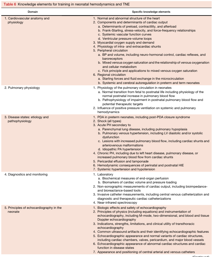
Table 6 Knowledge elements for training in neonatal hemodynamics and TNE <table><thead><tr><th>Domain</th><th>Specific knowledge elements</th></tr></thead><tbody><tr><td>1. Cardiovascular anatomy and physiology</td><td>1. Normal and abnormal structure of the heart<br>2. Components and determinants of cardiac output<br> a. Determinants of preload, contractility, and afterload<br> b. Frank-Starling, stress-velocity, and force-frequency relationships<br> c. Systemic vascular function curves<br> d. Ventricular pressure-volume loops<br>3. Myocardial oxygen supply and demand<br>4. Physiology of intra- and extracardiac shunts<br>5. Peripheral circulation<br> a. BP and volume, including neuro-hormonal control, cardiac reflexes, and baroreceptors<br> b. Mixed venous oxygen saturation and the relationship of venous oxygenation and cellular metabolism<br> c. Fick principle and applications to mixed venous oxygen saturation<br>6. Regional circulation<br> a. Starling forces and fluid exchange in the microcirculation<br> b. Systemic and cerebral autoregulation in preterm and term neonates</td></tr><tr><td>2. Pulmonary physiology</td><td>1. Physiology of the pulmonary circulation in neonates<br> a. Normal transition from fetal to postnatal life including physiology of the normal postnatal increase in pulmonary blood flow<br> b. Pathophysiology of impairment in postnatal pulmonary blood flow and potential therapeutic targets<br>2. Influence of positive pressure ventilation on systemic and pulmonary hemodynamics</td></tr><tr><td>3. Disease states: etiology and pathophysiology</td><td>1. PDA in preterm neonates, including post-PDA closure syndrome<br>2. Shock (all types)<br>3. Acute PH secondary to<br> a. Parenchymal lung disease, including pulmonary hypoplasia<br> b. Pulmonary venous hypertension, including LV diastolic and/or systolic dysfunction<br> c. Lesions with increased pulmonary blood flow, including cardiac shunts and arteriovenous malformations<br> d. Idiopathic PA hypertension<br>4. Chronic PH, including due to left heart disease, pulmonary disease, or increased pulmonary blood flow from cardiac shunts<br>5. Pericardial effusion and tamponade<br>6. Hemodynamic consequences of perinatal and postnatal HIE<br>7. Systemic hypertension and hypotension</td></tr><tr><td>4. Diagnostics and monitoring</td><td>1. Laboratory<br> a. Biochemical measures of end-organ perfusion<br> b. Biomarkers of cardiac volume and pressure loading<br>2. Non-sonographic measurements of cardiac output, including bioimpedance- and bioreactance-based tools<br>3. Invasive catheter measurements, including central venous catheterization and diagnostic and therapeutic cardiac catheterizations<br>4. Near-infrared spectroscopy</td></tr><tr><td>5. Principles of echocardiography in the neonate</td><td>1. Biologic effects and safety of echocardiography<br>2. Principles of physics (including equations) and instrumentation of echocardiography, including M-mode, two-dimensional, and blood and tissue Doppler echocardiography<br>3. Indications, strengths, limitations, and clinical utility of transthoracic echocardiography<br>4. Common ultrasound artifacts and their identifying echocardiographic features<br>5. Echocardiographic appearance and normal variants of cardiac structures, including cardiac chambers, valves, pericardium, and major blood vessels<br>6. Echocardiographic appearance of abnormal cardiac structures and cardiac function in disease states<br>7. Appearance and positioning of central arterial and venous catheters</td></tr></tbody></table>
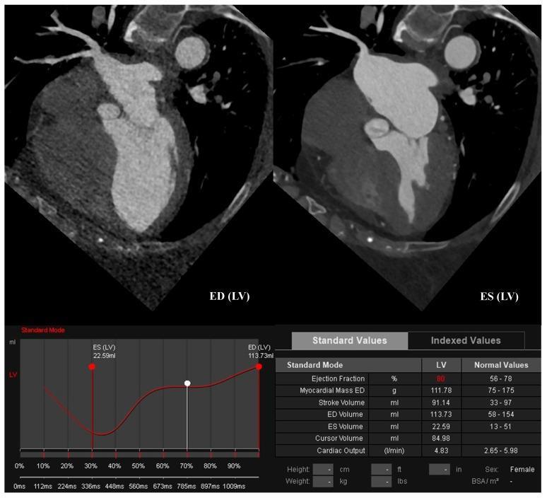
This diagnostic image displays a cardiac computed tomography angiography (CCTA) focused on left ventricular (LV) function assessment. The composite includes two side-by-side sagittal oblique views of the heart: the left frame shows the LV at end-diastole (ED), and the right frame shows it at end-systole (ES), illustrating the change in chamber volume during the cardiac cycle. Below the images is a quantitative analysis panel featuring a volume-time curve and a 'Standard Values' table. The data quantifies normal systolic function with an ejection fraction (EF) of 80%, a stroke volume (SV) of 91.14 mL, an end-diastolic volume (EDV) of 113.73 mL, and an end-systolic volume (ESV) of 22.59 mL. Additional parameters listed include a myocardial mass of 111.78 g and a cardiac output of 4.83 L/min. This clinical imaging tool is used in cardiology and radiology to objectively evaluate ventricular performance, wall motion, and myocardial health.
cardiac cycle pressure volume loop Wiggers diagram
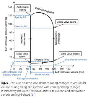
Summary : This figure shows a pressure–volume loop for the left ventricle, illustrating how ventricular volume and pressure change during the cardiac cycle, with key phases and valve events annotated. The isovolumetric relaxation and contraction periods are highlighted, and systolic/diastolic blood pressures are marked. pressure–volume loop diagram: # Title & Axes : • No explicit title on the figure, but the legend describes it as a "Pressure–volume loop demonstrating changes in ventricular volume during filling and ejection with corresponding changes in intracavity pressure." • X-axis: "Left ventricular volume (mL)" with tick marks at 0, 20, 40, 60, 80, 100, 120, 140, 160. • Y-axis: "Left ventricular pressure (mmHg)" with tick marks at 0, 20, 40, 60, 80, 100, 120, 140. • Additional axis labels: "Left ventricular end-diastolic pressure" (blue, left), "End-diastolic volume" (blue, bottom right), "Stroke volume" (black, bottom center). # Phases & Events : • Isovolumetric relaxation: vertical line at low volume, pressure drops, labeled. • Diastolic filling: horizontal line at low pressure, volume increases, labeled. • Isovolumetric contraction: vertical line at high volume, pressure rises, labeled. • Ventricular ejection: curved line, volume decreases as pressure peaks and falls, labeled. • Valve events: – Mitral valve opens (bottom left corner, low pressure/volume). – Mitral valve closes (bottom right corner, high volume/low pressure). – Aortic valve opens (top right corner, high volume/high pressure). – Aortic valve closes (top left corner, low volume/high pressure). # Blood Pressure Markers : • Systolic BP: horizontal dashed blue line at ~120 mmHg. • Diastolic BP: horizontal dashed blue line at ~80 mmHg. # Design Encodings : • Black solid lines for the loop. • Blue dashed lines for blood pressure markers. • Blue text for end-diastolic volume/pressure. • Labeled arrows for direction of phases and valve events. # Analysis : • The loop traces the cardiac cycle, starting at low pressure/volume (end-systolic), filling during diastole, rising sharply during isovolumetric contraction, ejecting blood during ventricular ejection, and dropping pressure during isovolumetric relaxation. • Systolic and diastolic blood pressures are marked, showing the pressure range during ejection. • The width of the loop (horizontal distance) represents stroke volume. • The figure clearly distinguishes the four main phases and the timing of valve openings/closings, providing a comprehensive view of ventricular mechanics during a heartbeat.
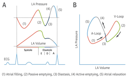
Summary : This figure illustrates the left atrial (LA) pressure-volume relationship during the cardiac cycle, showing both time-course traces and a pressure-volume loop, with key phases of atrial function annotated and correlated with the ECG. line plot and loop diagram: # Panel A: LA Pressure and Volume Traces • Top trace: LA Pressure (y-axis, arbitrary units) over time. • Middle trace: LA Volume (y-axis, arbitrary units) over time. • Bottom trace: ECG waveform for temporal reference. • X-axis: Cardiac cycle phases, with systole and diastole labeled; diastole further subdivided into E, D, and A phases. • Five phases are color-coded and numbered: – (1) Atrial filling (red) – (2) Passive emptying (green) – (3) Diastasis (black) – (4) Active emptying (blue) – (5) Atrial relaxation (gray) • Vertical dashed lines demarcate transitions between phases. # Panel B: LA Pressure-Volume Loop • X-axis: LA Volume (arbitrary units). • Y-axis: LA Pressure (arbitrary units). • The loop is traced in a counterclockwise direction, with arrows indicating the sequence. • The same five phases (1–5) are color-coded as in Panel A. • The loop is divided into two segments: A-Loop (phases 1, 3, 4, 5) and V-Loop (phase 2). # Design Encodings : • Distinct colors for each phase (red, green, black, blue, gray). • Arrows on the loop indicate the direction of the cardiac cycle. • ECG trace provides timing reference for the pressure and volume changes. # Analysis : • The LA pressure and volume traces show cyclical changes corresponding to atrial filling, emptying, and relaxation. • The pressure-volume loop visually summarizes the dynamic relationship between LA pressure and volume, with distinct segments for passive and active phases. • The figure highlights the temporal coordination between atrial events and the ECG, emphasizing the mechanical and electrical coupling in the cardiac cycle.
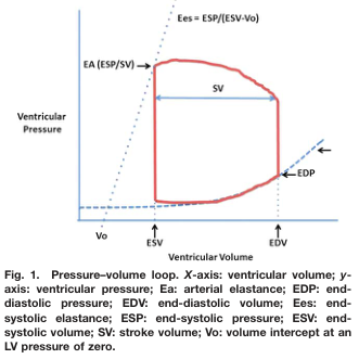
Summary : This figure presents a pressure–volume loop of the left ventricle, illustrating key cardiac parameters such as end-diastolic volume (EDV), end-systolic volume (ESV), stroke volume (SV), end-diastolic pressure (EDP), end-systolic pressure (ESP), arterial elastance (EA), and end-systolic elastance (Ees). The loop visually demonstrates the relationship between ventricular pressure and volume during a cardiac cycle. line plot: # Title & Axes : • Title: "Pressure–volume loop." • X-axis: "Ventricular Volume" (units not specified). – Tick labels: Vo (volume intercept at LV pressure of zero), ESV (end-systolic volume), EDV (end-diastolic volume). • Y-axis: "Ventricular Pressure" (units not specified). – No explicit tick labels shown. # Data & Curve : • Red closed loop traces the pressure–volume relationship during a cardiac cycle. • Horizontal arrow within the loop labeled "SV" (stroke volume) indicates the difference between EDV and ESV. • Vertical segments at EDV and ESV mark transitions between phases. • Dotted lines: – EA (arterial elastance) shown as a dashed line from Vo through ESP/SV. – Ees (end-systolic elastance) shown as a dashed line from Vo through ESP/(ESV-Vo). # Key Parameters & Annotations : • Vo: Volume intercept at LV pressure of zero (leftmost point on x-axis). • ESV: End-systolic volume (right vertical segment). • EDV: End-diastolic volume (far right on x-axis). • SV: Stroke volume (horizontal arrow between ESV and EDV). • EDP: End-diastolic pressure (arrow at bottom right of loop). • ESP: End-systolic pressure (top of loop). • EA: Arterial elastance (dashed line labeled EA (ESP/SV)). • Ees: End-systolic elastance (dashed line labeled Ees = ESP/(ESV-Vo)). # Design Encodings : • Red solid line for the pressure–volume loop. • Blue dashed lines for elastance relationships. • Arrows and labels for key parameters. • No gridlines or axis units specified. # Analysis : • The pressure–volume loop demonstrates the cardiac cycle phases, with the lower right corner representing end-diastole (high volume, low pressure) and the upper left corner representing end-systole (low volume, high pressure). • Stroke volume is visually indicated as the horizontal distance between EDV and ESV. • Elastance lines (EA and Ees) provide graphical representations of arterial and ventricular contractility. • The loop’s shape and annotations allow for assessment of cardiac function and mechanical properties.
mkdir -p /tmp/workspace/cardiac-physiology-ppt && ls /tmp/workspace/cardiac-physiology-ppt/
~/cardiac-physiology-ppt/build_ppt.py
import json
import subprocess
import base64
from io import BytesIO
from pptx import Presentation
from pptx.util import Inches, Pt, Emu
from pptx.dml.color import RGBColor
from pptx.enum.text import PP_ALIGN, MSO_ANCHOR
from pptx.util import Inches, Pt
# ── Colour palette ────────────────────────────────────────────────────────────
NAVY = RGBColor(0x0D, 0x2B, 0x55) # dark navy
MID_BLUE = RGBColor(0x1B, 0x4F, 0x8A) # header blue
ACCENT = RGBColor(0xE8, 0x4A, 0x30) # red-orange accent
LIGHT_BG = RGBColor(0xF4, 0xF7, 0xFC) # very light blue-white
WHITE = RGBColor(0xFF, 0xFF, 0xFF)
TEXT_DARK = RGBColor(0x1A, 0x1A, 0x2E)
GOLD = RGBColor(0xF0, 0xA5, 0x00)
TEAL = RGBColor(0x00, 0x7A, 0x87)
prs = Presentation()
prs.slide_width = Inches(13.333)
prs.slide_height = Inches(7.5)
blank = prs.slide_layouts[6]
# ── Helper: solid background rectangle ────────────────────────────────────────
def bg_rect(slide, color, left=0, top=0, width=None, height=None):
w = width if width is not None else prs.slide_width
h = height if height is not None else prs.slide_height
shape = slide.shapes.add_shape(1, left, top, w, h) # MSO_SHAPE_TYPE.RECTANGLE=1
fill = shape.fill
fill.solid()
fill.fore_color.rgb = color
shape.line.fill.background()
return shape
def add_text(slide, text, left, top, width, height,
font_name="Calibri", font_size=18, bold=False, italic=False,
color=WHITE, align=PP_ALIGN.LEFT, wrap=True, anchor=MSO_ANCHOR.TOP):
tb = slide.shapes.add_textbox(left, top, width, height)
tf = tb.text_frame
tf.word_wrap = wrap
tf.vertical_anchor = anchor
tf.margin_left = 0
tf.margin_right = 0
tf.margin_top = 0
tf.margin_bottom= 0
p = tf.paragraphs[0]
p.alignment = align
run = p.add_run()
run.text = text
run.font.name = font_name
run.font.size = Pt(font_size)
run.font.bold = bold
run.font.italic= italic
run.font.color.rgb = color
return tb
def add_multiline(slide, lines, left, top, width, height,
font_name="Calibri", font_size=16, bold=False,
color=TEXT_DARK, line_spacing_pt=4, bullet=True):
tb = slide.shapes.add_textbox(left, top, width, height)
tf = tb.text_frame
tf.word_wrap = True
tf.margin_left = Pt(2)
tf.margin_right = Pt(2)
tf.margin_top = Pt(4)
tf.margin_bottom = Pt(4)
first = True
for line in lines:
if first:
p = tf.paragraphs[0]
first = False
else:
p = tf.add_paragraph()
p.space_before = Pt(line_spacing_pt)
run = p.add_run()
run.text = ("• " if bullet else "") + line
run.font.name = font_name
run.font.size = Pt(font_size)
run.font.bold = bold
run.font.color.rgb = color
return tb
def header_bar(slide, title, subtitle=None):
"""Navy top bar with title and optional subtitle."""
bg_rect(slide, NAVY, 0, 0, prs.slide_width, Inches(1.25))
add_text(slide, title,
Inches(0.4), Inches(0.1), Inches(12.5), Inches(0.75),
font_size=30, bold=True, color=WHITE, anchor=MSO_ANCHOR.MIDDLE)
if subtitle:
add_text(slide, subtitle,
Inches(0.4), Inches(0.82), Inches(12.5), Inches(0.38),
font_size=15, italic=True, color=GOLD, anchor=MSO_ANCHOR.MIDDLE)
# thin accent line
line = slide.shapes.add_shape(1,
0, Inches(1.25), prs.slide_width, Pt(4))
line.fill.solid()
line.fill.fore_color.rgb = ACCENT
line.line.fill.background()
def footer(slide, slide_num, total=25):
bg_rect(slide, NAVY, 0, Inches(7.1), prs.slide_width, Inches(0.4))
add_text(slide, f"Cardiac Physiology | MD Residents | Slide {slide_num}/{total}",
Inches(0.3), Inches(7.1), Inches(12.7), Inches(0.4),
font_size=10, color=RGBColor(0xBB, 0xCC, 0xDD),
align=PP_ALIGN.CENTER, anchor=MSO_ANCHOR.MIDDLE)
def content_slide(slide, title, subtitle, bullet_lists, cols=1, image_url=None):
"""Generic 2-column or 1-column content slide with bullets."""
bg_rect(slide, LIGHT_BG)
header_bar(slide, title, subtitle)
content_top = Inches(1.35)
content_h = Inches(5.6)
if image_url and cols == 1:
cols = 2
if cols == 2:
col_w = Inches(6.3)
add_multiline(slide, bullet_lists[0],
Inches(0.3), content_top, col_w, content_h,
font_size=15, color=TEXT_DARK)
if image_url:
try:
result = json.loads(subprocess.check_output(
["python", "/tmp/skills/shared/scripts/fetch_images.py", image_url],
timeout=30
))
if result and result[0]["base64"]:
raw = base64.b64decode(result[0]["base64"].split(",",1)[1])
slide.shapes.add_picture(BytesIO(raw),
Inches(6.8), content_top, col_w, content_h - Inches(0.3))
except Exception as e:
add_text(slide, f"[Image unavailable: {e}]",
Inches(6.8), content_top, col_w, content_h,
font_size=12, color=TEXT_DARK)
elif len(bullet_lists) > 1:
add_multiline(slide, bullet_lists[1],
Inches(6.8), content_top, col_w, content_h,
font_size=15, color=TEXT_DARK)
else:
add_multiline(slide, bullet_lists[0],
Inches(0.3), content_top, Inches(12.7), content_h,
font_size=15, color=TEXT_DARK)
def two_col_text(slide, title, subtitle, left_bullets, right_bullets):
bg_rect(slide, LIGHT_BG)
header_bar(slide, title, subtitle)
top = Inches(1.35)
h = Inches(5.6)
col_w = Inches(6.3)
add_multiline(slide, left_bullets, Inches(0.3), top, col_w, h, font_size=15, color=TEXT_DARK)
add_multiline(slide, right_bullets, Inches(6.8), top, col_w, h, font_size=15, color=TEXT_DARK)
# ══════════════════════════════════════════════════════════════════════════════
# SLIDE DATA
# ══════════════════════════════════════════════════════════════════════════════
slides_data = []
# ── 1. TITLE ──────────────────────────────────────────────────────────────────
def make_slide_1():
s = prs.slides.add_slide(blank)
bg_rect(s, NAVY)
# large decorative circle
circ = s.shapes.add_shape(9, Inches(9.5), Inches(-1), Inches(6), Inches(6)) # OVAL=9
circ.fill.solid()
circ.fill.fore_color.rgb = MID_BLUE
circ.line.fill.background()
add_text(s, "CARDIAC PHYSIOLOGY",
Inches(0.6), Inches(1.5), Inches(8), Inches(1.2),
font_size=44, bold=True, color=WHITE, align=PP_ALIGN.LEFT)
add_text(s, "A Comprehensive Review for MD Residents",
Inches(0.6), Inches(2.8), Inches(8), Inches(0.6),
font_size=22, italic=True, color=GOLD)
add_text(s, "Topics: Cardiac Anatomy & Muscle • Action Potentials • Conduction System\n"
"Cardiac Cycle • Haemodynamics • Contractility • Autonomic Regulation\n"
"Coronary Circulation • Heart Failure Physiology",
Inches(0.6), Inches(3.6), Inches(8.5), Inches(1.6),
font_size=14, color=RGBColor(0xCC, 0xDD, 0xFF))
# divider
div = s.shapes.add_shape(1, Inches(0.6), Inches(3.45), Inches(7), Pt(3))
div.fill.solid(); div.fill.fore_color.rgb = ACCENT; div.line.fill.background()
add_text(s, "Sources: Guyton & Hall • Miller's Anesthesia • Sabiston Surgery",
Inches(0.6), Inches(5.4), Inches(8), Inches(0.4),
font_size=11, color=RGBColor(0x88, 0xAA, 0xCC))
footer(s, 1)
make_slide_1()
# ── 2. OVERVIEW / AGENDA ──────────────────────────────────────────────────────
def make_slide_2():
s = prs.slides.add_slide(blank)
bg_rect(s, LIGHT_BG)
header_bar(s, "Lecture Outline", "25-Slide Overview")
topics = [
("1–3", "Cardiac Anatomy & Muscle Ultrastructure"),
("4–5", "Excitation-Contraction Coupling & Calcium"),
("6–7", "Cardiac Action Potentials (Working & Pacemaker)"),
("8–9", "Conduction System & ECG Correlation"),
("10–11","Cardiac Cycle: Phases & Valve Events"),
("11–12","Pressure-Volume Loops"),
("13–14","Determinants of Cardiac Output"),
("15–16","Frank-Starling Mechanism & Preload"),
("17–18","Afterload, Contractility & Laplace's Law"),
("19–20","Autonomic Regulation (SNS / PSNS)"),
("21–22","Coronary Circulation & O₂ Demand"),
("23–24","Integrated Hemodynamics & Heart Failure"),
("25", "Summary, Key Equations & Clinical Pearls"),
]
left_col = topics[:7]
right_col = topics[7:]
top = Inches(1.4)
for i, (nums, topic) in enumerate(left_col):
y = top + Inches(i * 0.74)
# pill background
pill = s.shapes.add_shape(1, Inches(0.3), y, Inches(0.75), Inches(0.45))
pill.fill.solid(); pill.fill.fore_color.rgb = MID_BLUE; pill.line.fill.background()
add_text(s, nums, Inches(0.3), y, Inches(0.75), Inches(0.45),
font_size=10, bold=True, color=WHITE, align=PP_ALIGN.CENTER, anchor=MSO_ANCHOR.MIDDLE)
add_text(s, topic, Inches(1.15), y, Inches(5.4), Inches(0.45),
font_size=13, color=TEXT_DARK, anchor=MSO_ANCHOR.MIDDLE)
for i, (nums, topic) in enumerate(right_col):
y = top + Inches(i * 0.74)
pill = s.shapes.add_shape(1, Inches(6.8), y, Inches(0.75), Inches(0.45))
pill.fill.solid(); pill.fill.fore_color.rgb = TEAL; pill.line.fill.background()
add_text(s, nums, Inches(6.8), y, Inches(0.75), Inches(0.45),
font_size=10, bold=True, color=WHITE, align=PP_ALIGN.CENTER, anchor=MSO_ANCHOR.MIDDLE)
add_text(s, topic, Inches(7.65), y, Inches(5.4), Inches(0.45),
font_size=13, color=TEXT_DARK, anchor=MSO_ANCHOR.MIDDLE)
footer(s, 2)
make_slide_2()
# ── 3. CARDIAC ANATOMY OVERVIEW ───────────────────────────────────────────────
def make_slide_3():
s = prs.slides.add_slide(blank)
bg_rect(s, LIGHT_BG)
header_bar(s, "Cardiac Anatomy: Functional Overview", "Four Chambers, Two Circulations")
two_col_text(s, "Cardiac Anatomy: Functional Overview", "Four Chambers, Two Circulations",
[
"Right heart: low-pressure pulmonary circuit",
"Left heart: high-pressure systemic circuit",
"Two atria → thin-walled, low pressure (~5–10 mmHg)",
"Two ventricles → thick-walled, high pressure",
"LV wall ~3× thicker than RV (≈9 mm vs 3 mm)",
"Interventricular septum shared by both ventricles",
"Four fibrous valves prevent retrograde flow",
"AV valves: Mitral (bicuspid), Tricuspid",
"Semilunar valves: Aortic, Pulmonary",
],
[
"Pericardium: fibrous sac limits overdistension",
"Epicardium = visceral pericardium",
"Myocardium: working muscle of heart",
"Endocardium: inner lining, forms valves",
"Coronary arteries arise from aortic sinuses",
"Right coronary → RV + inferior LV + SA/AV nodes",
"Left main → LAD + LCx (lateral/anterior LV)",
"Venous return: coronary sinus → right atrium",
"Cardiac lymphatics → mediastinal lymph nodes",
])
footer(s, 3)
make_slide_3()
# ── 4. CARDIAC MUSCLE ULTRASTRUCTURE ─────────────────────────────────────────
def make_slide_4():
s = prs.slides.add_slide(blank)
bg_rect(s, LIGHT_BG)
header_bar(s, "Cardiac Muscle Ultrastructure", "Sarcomere → Syncytium")
two_col_text(s, "Cardiac Muscle Ultrastructure", "Sarcomere → Syncytium",
[
"Cardiomyocytes: branched, striated, uninucleate",
"Sarcomere (1.6–2.2 µm): basic contractile unit",
"Thin filaments: actin + troponin + tropomyosin",
"Thick filaments: myosin heavy chains (β-MHC dominant in ventricle)",
"Z-disc anchors thin filaments",
"M-line anchors thick filaments",
"I-band: thin filaments only",
"A-band: thick (+ overlap) — constant length",
"Titin: elastic spring, determines passive stiffness",
],
[
"Intercalated discs connect cells end-to-end",
"Fascia adherens: mechanical coupling (connects actin)",
"Desmosomes: resist shearing forces",
"Gap junctions (connexin-43): electrical coupling",
"→ Functional syncytium: whole atria / ventricles contract together",
"T-tubules: deep invaginations at Z-discs",
"Sarcoplasmic reticulum: Ca²⁺ storage reservoir",
"High mitochondria density (~30% cell volume) for ATP",
"Cardiac muscle CANNOT regenerate (terminally differentiated)",
])
footer(s, 4)
make_slide_4()
# ── 5. EXCITATION-CONTRACTION COUPLING ───────────────────────────────────────
def make_slide_5():
s = prs.slides.add_slide(blank)
bg_rect(s, LIGHT_BG)
header_bar(s, "Excitation-Contraction Coupling", "The Central Role of Calcium")
two_col_text(s, "Excitation-Contraction Coupling", "The Central Role of Calcium",
[
"Action potential → depolarises T-tubule membrane",
"L-type Ca²⁺ channels (LTCC / Cav1.2) open",
"Trigger Ca²⁺ influx (~10% of total Ca²⁺)",
"Ca²⁺ binds RyR2 (ryanodine receptor) on SR",
"CICR: Ca²⁺-induced Ca²⁺ release from SR (90%)",
"Cytosolic Ca²⁺ rises: ~0.1 µM → ~1 µM",
"Ca²⁺ binds troponin C → conformational change",
"Tropomyosin shifts → actin-myosin cross-bridges form",
],
[
"Cross-bridge cycling: power stroke → ADP+Pi released",
"ATP required for detachment of myosin head",
"Rigor mortis = no ATP → cross-bridges locked",
"Relaxation: Ca²⁺ pumped back by:",
" → SERCA2a (SR Ca-ATPase): 70% reuptake",
" → NCX (Na⁺-Ca²⁺ exchanger): extrudes Ca²⁺",
" → Sarcolemmal Ca-ATPase (minor)",
"PLB (phospholamban) inhibits SERCA2a",
"PKA phosphorylates PLB → relieves inhibition → faster relaxation (lusitropy)",
])
footer(s, 5)
make_slide_5()
# ── 6. ACTION POTENTIAL — WORKING MYOCYTE ─────────────────────────────────────
def make_slide_6():
s = prs.slides.add_slide(blank)
bg_rect(s, LIGHT_BG)
header_bar(s, "Ventricular Action Potential", "5 Phases — Working Myocyte")
two_col_text(s, "Ventricular Action Potential", "5 Phases — Working Myocyte",
[
"Phase 0 — Rapid depolarisation",
" INa (fast Na⁺ influx): RMP −90 mV → +30 mV",
" Threshold ≈ −70 mV; rises at 300 V/s",
"",
"Phase 1 — Rapid initial repolarisation",
" INa inactivation + Ito (transient K⁺ outward)",
" 'Notch' seen on ventricular AP",
"",
"Phase 2 — Plateau (unique to cardiac muscle!)",
" ICa-L (slow Ca²⁺ in) ≈ IKr/IKs (K⁺ out)",
" ~200–400 ms — prevents tetanic contraction",
],
[
"Phase 3 — Rapid repolarisation",
" IKr + IKs (rapid & slow delayed K⁺ channels)",
" Ca²⁺ channels inactivate",
" Returns to −90 mV",
"",
"Phase 4 — Resting membrane potential",
" −90 mV maintained by IK1 (inward rectifier)",
" No spontaneous depolarisation in working cells",
"",
"Effective Refractory Period (ERP): phases 0–3",
" Cannot re-excite during AP → protective",
" Long ERP prevents summation/tetanus",
"QT interval on ECG ≈ AP duration",
])
footer(s, 6)
make_slide_6()
# ── 7. PACEMAKER ACTION POTENTIAL ─────────────────────────────────────────────
def make_slide_7():
s = prs.slides.add_slide(blank)
bg_rect(s, LIGHT_BG)
header_bar(s, "Pacemaker Action Potential", "SA Node — Automaticity & Spontaneous Depolarisation")
two_col_text(s, "Pacemaker Action Potential", "SA Node — Automaticity & Spontaneous Depolarisation",
[
"SA node RMP: −60 mV (less negative than working cells)",
"No true stable resting potential",
"Phase 4: Spontaneous ('funny') depolarisation",
" If (funny current) → HCN channels → Na⁺/K⁺ influx",
" Slow Ca²⁺ leak (T-type Ca channels) contributes",
"Threshold ≈ −40 mV",
"Phase 0: Slow upstroke via ICaL (NOT INa)",
" Slow rise → slow conduction velocity",
],
[
"Phase 3: Repolarisation via IK channels",
"No plateau phase in SA/AV nodal cells",
"Intrinsic rate: SA ~60–100 bpm | AV ~40–60 | HPS ~20–40",
"SA node dominates (fastest automaticity) → pacemaker",
"SNS → ↑If + ↑ICaL → ↑heart rate (positive chronotropy)",
"PSNS (M2 receptors) → ↑IKACh → hyperpolarise → ↓HR",
"Overdrive suppression: faster pacemaker suppresses slower",
"Clinical: β-blockers act on SA node (negative chronotropy)",
"Ivabradine: selectively blocks If → ↓HR, ↓O₂ demand",
])
footer(s, 7)
make_slide_7()
# ── 8. CONDUCTION SYSTEM ──────────────────────────────────────────────────────
def make_slide_8():
s = prs.slides.add_slide(blank)
bg_rect(s, LIGHT_BG)
header_bar(s, "Cardiac Conduction System", "SA Node → Purkinje Fibres")
two_col_text(s, "Cardiac Conduction System", "SA Node → Purkinje Fibres",
[
"1. SA Node (sinoatrial): crista terminalis, RA",
" Dominant pacemaker; rate 60–100 bpm",
"2. Internodal tracts: Bachmann's bundle (to LA)",
"3. AV Node: interatrial septum",
" KEY delay: 0.12–0.20 s (PR interval)",
" Only normal AV conduction pathway",
" Decremental conduction → prevents AF → VF",
" Blood supply: RCA (90%), LCx (10%)",
],
[
"4. Bundle of His: penetrates fibrous skeleton",
"5. Left Bundle Branch (LBB): anterior + posterior fascicles",
"6. Right Bundle Branch (RBB): single fascicle",
"7. Purkinje fibres: subendocardial plexus",
" Fastest conduction: 4 m/s (vs AV node 0.05 m/s)",
" Endocardium → epicardium activation",
" Apex → base direction of contraction",
"ECG correlations: PR = AV conduction, QRS = ventricular depol,",
"QT = AP duration, ST = plateau phase, T = repolarisation",
])
footer(s, 8)
make_slide_8()
# ── 9. ECG & CONDUCTION CORRELATION ───────────────────────────────────────────
def make_slide_9():
s = prs.slides.add_slide(blank)
bg_rect(s, LIGHT_BG)
header_bar(s, "ECG Correlation with Conduction", "Electrical Events & Normal Intervals")
two_col_text(s, "ECG Correlation with Conduction", "Electrical Events & Normal Intervals",
[
"P wave: atrial depolarisation (SA → AV node)",
"PR interval: 0.12–0.20 s (AV nodal delay)",
" ↑PR = 1st degree AV block",
"QRS complex: ventricular depolarisation",
" Normal <0.12 s; BBB >0.12 s",
"ST segment: ventricular plateau phase",
" ST elevation → STEMI; ST depression → ischaemia",
"T wave: ventricular repolarisation",
"QT interval: total AP duration; corrected QTc",
" QTc > 440 ms (men), >460 ms (women) = prolonged",
],
[
"U wave: Purkinje repolarisation or hypokalemia",
"Axis: normal −30° to +90°; LAD, RAD",
"Vectors: depolarisation travels toward positive electrode",
"Leads I, aVL: lateral; II, III, aVF: inferior",
"V1–V2: septal; V3–V4: anterior; V5–V6: lateral",
"Brugada pattern: RBBB + ST elevation V1–V3",
"LVH: Sokolow-Lyon index > 35 mm",
"Delta wave (WPW): pre-excitation via accessory pathway",
"Ashman phenomenon: aberrant conduction after long-short",
"Clinical: 12-lead ECG = indispensable physiology tool",
])
footer(s, 9)
make_slide_9()
# ── 10. CARDIAC CYCLE — PHASES ────────────────────────────────────────────────
def make_slide_10():
s = prs.slides.add_slide(blank)
bg_rect(s, LIGHT_BG)
header_bar(s, "The Cardiac Cycle", "Sequential Mechanical Events During One Heartbeat")
phases = [
("DIASTOLE", MID_BLUE, [
"1. Isovolumetric Relaxation",
" Aortic valve closes (dicrotic notch)",
" AV valves still closed; pressure drops",
" Duration ~70 ms",
"2. Rapid Ventricular Filling",
" Mitral/tricuspid opens when LVP < LAP",
" ~80% filling; E-wave on echo",
"3. Diastasis (slow filling)",
" Minimal flow; plateau",
"4. Atrial Contraction ('atrial kick')",
" ~20% of filling; A-wave; contributes to late filling",
" Absent in AF → ↓CO 20–30% in stiff ventricles",
]),
("SYSTOLE", ACCENT, [
"5. Isovolumetric Contraction",
" AV valves close (S1); all valves closed",
" LVP rises without change in volume",
" Duration ~50–60 ms",
"6. Rapid Ejection",
" Aortic valve opens when LVP > aortic P",
" ~70% of SV ejected rapidly",
"7. Reduced Ejection",
" Slowing ejection as AV pressure equalises",
" S2 = aortic + pulmonary valve closure",
" EF = SV/EDV × 100%; normal ≥55%",
]),
]
col_x = [Inches(0.3), Inches(6.8)]
for ci, (label, col_color, bullets) in enumerate(phases):
lbl = s.shapes.add_shape(1, col_x[ci], Inches(1.38), Inches(6.2), Inches(0.45))
lbl.fill.solid(); lbl.fill.fore_color.rgb = col_color; lbl.line.fill.background()
add_text(s, label, col_x[ci], Inches(1.38), Inches(6.2), Inches(0.45),
font_size=14, bold=True, color=WHITE, align=PP_ALIGN.CENTER, anchor=MSO_ANCHOR.MIDDLE)
add_multiline(s, bullets, col_x[ci], Inches(1.9), Inches(6.2), Inches(5.1),
font_size=13, color=TEXT_DARK, bullet=False)
footer(s, 10)
make_slide_10()
# ── 11. PRESSURE-VOLUME LOOP ──────────────────────────────────────────────────
def make_slide_11():
s = prs.slides.add_slide(blank)
bg_rect(s, LIGHT_BG)
header_bar(s, "Pressure-Volume Loop", "Left Ventricular Mechanics")
img = "https://cdn.orris.care/cdss_images/GLGCA_4716091_1766472503888_9982bb46-edd6-4c5b-96d5-780f4569c406_39a92e8d-bdef-4225-b8d7-22f263ffa161.png"
try:
result = json.loads(subprocess.check_output(
["python", "/tmp/skills/shared/scripts/fetch_images.py", img], timeout=30))
if result and result[0]["base64"]:
raw = base64.b64decode(result[0]["base64"].split(",",1)[1])
s.shapes.add_picture(BytesIO(raw), Inches(0.3), Inches(1.35), Inches(6.2), Inches(5.7))
except Exception as e:
add_text(s, "[P-V loop image]", Inches(0.3), Inches(1.35), Inches(6.2), Inches(5.7), font_size=12, color=TEXT_DARK)
add_multiline(s, [
"Loop width = Stroke Volume (EDV − ESV)",
"Loop height = systolic pressure range",
"Slope of ESPVR (Ees) = contractility index",
"EA (arterial elastance) = afterload",
"Efficiency = stroke work / pressure-volume area",
"↑ Preload → loop shifts right (wider)",
"↑ Afterload → loop taller, narrower (↓SV)",
"↑ Contractility → loop shifts left (↑SV + ↑ESP)",
"LVEDP = end-diastolic pressure (preload surrogate)",
"EDV normal: 120–130 mL; ESV: 50–60 mL",
"EF = SV/EDV = (EDV−ESV)/EDV; normal ≥55%",
"Ventriculo-arterial coupling: optimal when Ees/EA ≈ 1",
], Inches(6.8), Inches(1.35), Inches(6.2), Inches(5.7),
font_size=14, color=TEXT_DARK)
footer(s, 11)
make_slide_11()
# ── 12. CARDIAC OUTPUT & ITS DETERMINANTS ─────────────────────────────────────
def make_slide_12():
s = prs.slides.add_slide(blank)
bg_rect(s, LIGHT_BG)
header_bar(s, "Cardiac Output & Its Determinants", "CO = HR × SV")
two_col_text(s, "Cardiac Output & Its Determinants", "CO = HR × SV",
[
"Cardiac Output (CO) = HR × Stroke Volume",
"Normal at rest: 5 L/min (range 4–8 L/min)",
"Cardiac Index (CI) = CO / BSA; normal 2.5–4.0 L/min/m²",
"",
"HEART RATE (HR)",
" Normal: 60–100 bpm",
" SNS → ↑HR; PSNS → ↓HR",
" At very high HR: ↓diastolic filling → ↓SV",
" CO peaks at ~120 bpm; falls above",
"",
"STROKE VOLUME (SV)",
" SV = EDV − ESV (normal ~70 mL)",
" 3 determinants: Preload, Afterload, Contractility",
],
[
"Mixed Venous O₂ sat (SvO₂) reflects CO adequacy",
" Normal SvO₂: 65–75%",
" Low SvO₂ → ↑O₂ extraction → inadequate CO",
"",
"Fick Principle:",
" CO = VO₂ / (CaO₂ − CvO₂)",
" Gold standard for CO measurement",
"",
"Thermodilution (PA catheter): clinical standard",
" Overcomes Fick's need for VO₂ measurement",
"",
"Measured CO values:",
" Septic shock: hyperdynamic ↑CO",
" Cardiogenic shock: ↓CO, ↑SVR",
" Heart failure: ↓CO at rest or with stress",
])
footer(s, 12)
make_slide_12()
# ── 13. PRELOAD ───────────────────────────────────────────────────────────────
def make_slide_13():
s = prs.slides.add_slide(blank)
bg_rect(s, LIGHT_BG)
header_bar(s, "Preload", "Ventricular End-Diastolic Volume & Filling Pressure")
two_col_text(s, "Preload", "Ventricular End-Diastolic Volume & Filling Pressure",
[
"Definition: myocardial fibre stretch at END of diastole",
"Best measure: LVEDV (clinical surrogate: LVEDP, PCWP)",
"Normal LVEDP: 8–12 mmHg",
"Normal LVEDV: 120–130 mL",
"",
"Determinants of Preload:",
" Venous return (most important)",
" Total blood volume",
" Venous tone (venous capacitance)",
" Intrathoracic pressure (negative → enhances filling)",
" Heart rate (↑HR → ↓filling time → ↓preload)",
" Atrial contraction (adds 20% to filling)",
" Pericardial constraint",
],
[
"Starling's Law: ↑preload → ↑force of contraction",
"Mechanism: ↑sarcomere length → optimal actin-myosin overlap",
" → ↑Ca²⁺ sensitivity of troponin C",
" → ↑cross-bridge formation",
"Optimal sarcomere length: 2.2 µm",
"",
"Clinical assessment of preload:",
" JVP / CVP (right heart)",
" PCWP via PA catheter (left heart)",
" Echo: LVEDD, E/A ratio",
" IVC collapsibility index",
"",
"Fluid challenge: standard method to assess preload responsiveness",
"Passive Leg Raise (PLR): reversible, safe preload test",
])
footer(s, 13)
make_slide_13()
# ── 14. FRANK-STARLING MECHANISM ──────────────────────────────────────────────
def make_slide_14():
s = prs.slides.add_slide(blank)
bg_rect(s, LIGHT_BG)
header_bar(s, "Frank-Starling Mechanism", "The Heart's Intrinsic Autoregulation")
img = "https://cdn.orris.care/cdss_images/GLGCA_11173_1762898798398_6b9c785a-c63f-46c2-bb11-d9bae18f8286.png"
try:
result = json.loads(subprocess.check_output(
["python", "/tmp/skills/shared/scripts/fetch_images.py", img], timeout=30))
if result and result[0]["base64"]:
raw = base64.b64decode(result[0]["base64"].split(",",1)[1])
s.shapes.add_picture(BytesIO(raw), Inches(0.3), Inches(1.35), Inches(6.2), Inches(5.7))
except:
add_text(s, "[Frank-Starling curve]", Inches(0.3), Inches(1.35), Inches(6.2), Inches(5.7), font_size=12, color=TEXT_DARK)
add_multiline(s, [
"Law: the greater the filling (EDV), the greater the force",
" of contraction → ↑SV",
"Molecular basis: length-dependent Ca²⁺ activation",
" ↑SL → reduced inter-filament spacing → ↑troponin C affinity",
"Self-regulating: equalises output of right and left hearts",
"Ascending limb: increasing EDV → ↑SV (physiologic range)",
"Plateau: optimal sarcomere length reached",
"Descending limb: rarely reached in intact heart",
"↑Contractility → curve shifts UP & LEFT",
"Heart failure → curve shifts DOWN & RIGHT",
"Heterometric regulation = Starling mechanism",
"Homeometric regulation = Anrep effect (↑afterload → ↑inotropy)",
], Inches(6.8), Inches(1.35), Inches(6.2), Inches(5.7),
font_size=14, color=TEXT_DARK)
footer(s, 14)
make_slide_14()
# ── 15. AFTERLOAD ─────────────────────────────────────────────────────────────
def make_slide_15():
s = prs.slides.add_slide(blank)
bg_rect(s, LIGHT_BG)
header_bar(s, "Afterload", "Wall Stress During Ejection — Laplace's Law")
two_col_text(s, "Afterload", "Wall Stress During Ejection — Laplace's Law",
[
"Definition: load against which ventricle ejects blood",
"Best measure: wall stress = (P × r) / (2 × h)",
" P = intracavitary pressure; r = radius; h = wall thickness",
" Laplace's Law: as r↑ or P↑ → wall stress↑",
"",
"Clinical surrogates of afterload:",
" SVR = (MAP − CVP) / CO × 80 (dynes·s·cm⁻⁵)",
" Normal SVR: 800–1200 dynes·s·cm⁻⁵",
" Aortic impedance (most accurate)",
"",
"Effect of ↑Afterload:",
" ↑Wall stress → ↓fibre shortening velocity → ↓SV",
" Compensatory: ↑EDV (Starling) buffers ↓SV",
" Chronic ↑afterload → concentric LV hypertrophy",
],
[
"Laplace & Dilated Cardiomyopathy:",
" ↑r (dilated LV) → ↑wall stress even at normal pressures",
" Oxygen demand↑; ischaemia risk↑",
"",
"Afterload reduction therapy:",
" ACE inhibitors / ARBs → vasodilation → ↓SVR",
" Hydralazine → arteriolar dilation",
" Nitroprusside → arterial + venous dilation",
" Amlodipine → Ca channel block → vasodilation",
"",
"Right ventricle afterload:",
" PVR = (mPAP − PCWP) / CO × 80",
" Normal PVR: 100–250 dynes·s·cm⁻⁵",
" Pulmonary HTN → ↑RV afterload → RV failure",
])
footer(s, 15)
make_slide_15()
# ── 16. CONTRACTILITY ─────────────────────────────────────────────────────────
def make_slide_16():
s = prs.slides.add_slide(blank)
bg_rect(s, LIGHT_BG)
header_bar(s, "Myocardial Contractility (Inotropy)", "Intrinsic Force of Contraction")
two_col_text(s, "Myocardial Contractility (Inotropy)", "Intrinsic Force of Contraction",
[
"Definition: intrinsic ability of myocardium to generate force",
"Independent of preload and afterload",
"Best index: Ees (end-systolic elastance, slope of ESPVR)",
"Clinical: dP/dt max, EF (affected by load), MAPSE, GLS",
"",
"↑Contractility (Positive inotropy):",
" β₁-adrenergic activation → ↑cAMP → PKA",
" PKA phosphorylates LTCC → ↑Ca²⁺ entry",
" PKA phosphorylates PLB → ↑SERCA2a → faster relaxation",
" Catecholamines, dobutamine, dopamine",
" Digoxin: inhibits Na⁺/K⁺-ATPase → ↑intracellular Na⁺",
" → ↓NCX activity → ↑intracellular Ca²⁺",
" Milrinone: PDE3 inhibitor → ↑cAMP",
],
[
"↓Contractility (Negative inotropy):",
" β-blockers, Ca²⁺ channel blockers",
" Myocardial ischaemia / infarction",
" Metabolic acidosis (↑H⁺ → ↓troponin Ca affinity)",
" Hypoxia, hypercapnia",
" Negative inotropes: volatile anaesthetics",
"",
"Treppe / Bowditch effect:",
" ↑HR → ↑contractility (force-frequency relationship)",
" More Ca²⁺ accumulates with faster pacing",
"",
"β₁ receptor signalling:",
" Gs → adenylyl cyclase → ↑cAMP",
" PKA → LTCC, PLB, troponin I (lusitropic effect)",
" Heart failure: β₁ receptor downregulation",
])
footer(s, 16)
make_slide_16()
# ── 17. AUTONOMIC REGULATION OF HEART RATE & CONTRACTILITY ────────────────────
def make_slide_17():
s = prs.slides.add_slide(blank)
bg_rect(s, LIGHT_BG)
header_bar(s, "Autonomic Regulation", "Sympathetic & Parasympathetic Control")
two_col_text(s, "Autonomic Regulation", "Sympathetic & Parasympathetic Control",
[
"SYMPATHETIC (fight-or-flight)",
" Preganglionic: T1–T4 → superior/middle/inferior cardiac nerves",
" Neurotransmitter: norepinephrine (NE)",
" Receptors: β₁ (dominant), β₂, α₁",
" β₁ effects:",
" Chronotropy: ↑HR (↑If in SA node)",
" Inotropy: ↑contractility (PKA cascade)",
" Lusitropy: ↑relaxation speed",
" Dromotropy: ↑AV conduction velocity",
" α₁: arteriolar constriction → ↑SVR",
" Circulating catecholamines (adrenal medulla) amplify",
],
[
"PARASYMPATHETIC (rest-and-digest)",
" Cranial nerve X (vagus) → cardiac branches",
" Dense innervation to SA + AV nodes (atria > ventricles)",
" Neurotransmitter: acetylcholine (ACh)",
" Receptors: M₂ (muscarinic)",
" M₂ effects:",
" ↑IKACh → hyperpolarisation → ↓HR (negative chronotropy)",
" ↓AV node conduction → ↑PR interval",
" Mild negative inotropy (atria > ventricle)",
" Resting tone: vagal dominance → HR < intrinsic SA rate",
" Atropine: blocks M₂ → ↑HR (used in bradycardia)",
" Baroreflex: ↑MAP → ↑vagal tone → ↓HR",
])
footer(s, 17)
make_slide_17()
# ── 18. BARORECEPTOR REFLEX ────────────────────────────────────────────────────
def make_slide_18():
s = prs.slides.add_slide(blank)
bg_rect(s, LIGHT_BG)
header_bar(s, "Baroreflex & Neural Control of Circulation", "Short-Term Blood Pressure Regulation")
two_col_text(s, "Baroreflex & Neural Control of Circulation", "Short-Term Blood Pressure Regulation",
[
"Arterial baroreceptors: carotid sinus (CN IX), aortic arch (CN X)",
"Detect wall stretch proportional to MAP",
"Fire continuously; ↑MAP → ↑firing rate",
"Afferent signals → NTS in medulla",
"",
"Cardiovascular control centre (medulla):",
" Vasomotor centre (C1 neurons): tonically active → SNS",
" Vagal dorsal motor nucleus / NA → PSNS efferents",
"",
"Normal blood pressure set-point: ~100 mmHg MAP",
"Response to ↑MAP:",
" ↑Vagal tone → ↓HR (neg. chronotropy)",
" ↓Sympathetic tone → ↓SVR → ↓MAP",
" Response within 5–10 seconds",
],
[
"Response to ↓MAP (haemorrhage, standing):",
" ↓Baroreceptor firing → ↑SNS, ↓PSNS",
" ↑HR, ↑contractility, ↑SVR",
" Vasoconstriction → ↑venous return",
"",
"Cardiopulmonary receptors (low-pressure):",
" Atrial stretch receptors (Bainbridge reflex)",
" ↑Atrial filling → ↑HR (reflex tachycardia)",
" ↑ADH release → ↑water retention",
"",
"Chemoreceptor reflex:",
" Central (medullary): ↑PCO₂/↑H⁺ → ↑ventilation + ↑HR",
" Peripheral (carotid/aortic bodies): ↓PO₂ → ↑HR, ↑ventilation",
"",
"Cushing reflex: ↑ICP → HTN + bradycardia (Cushing's triad)",
"Clinical: orthostatic hypotension = baroreflex failure",
])
footer(s, 18)
make_slide_18()
# ── 19. CORONARY CIRCULATION ──────────────────────────────────────────────────
def make_slide_19():
s = prs.slides.add_slide(blank)
bg_rect(s, LIGHT_BG)
header_bar(s, "Coronary Circulation", "O₂ Supply–Demand Balance")
two_col_text(s, "Coronary Circulation", "O₂ Supply–Demand Balance",
[
"Coronary blood flow (CBF): ~250 mL/min at rest (~5% CO)",
"LV flow: mainly during DIASTOLE (systolic compression)",
"RV flow: throughout cardiac cycle (lower wall stress)",
"Coronary perfusion pressure = Diastolic BP − LVEDP",
"Tachycardia → ↓diastolic time → ↑ischaemia risk",
"",
"O₂ SUPPLY determinants:",
" Coronary blood flow (perfusion pressure / vascular resistance)",
" Arterial O₂ content (CaO₂ = Hb × 1.34 × SaO₂)",
" O₂ extraction already ~75% at rest (vs skeletal 25%)",
" → ↑demand met almost entirely by ↑CBF, not ↑extraction",
],
[
"O₂ DEMAND determinants (MVO₂):",
" Heart rate (most important!)",
" Wall stress (preload + afterload: Laplace)",
" Contractility (inotropy)",
" Basal metabolic rate (minor)",
" Double product = HR × SBP (clinical O₂ demand index)",
"",
"Coronary autoregulation: maintains CBF constant",
" MAP 60–140 mmHg → myogenic + metabolic mechanisms",
" Adenosine (most potent): released with ↑work → vasodilation",
" NO, prostacyclin, K⁺ also mediate metabolic hyperaemia",
"",
"Coronary steal: vasodilators (dipyridamole, adenosine)",
" → preferential dilation of normal vessels",
" → ↓flow to ischaemic territories (steal)",
])
footer(s, 19)
make_slide_19()
# ── 20. VENOUS RETURN & GUYTON CURVES ─────────────────────────────────────────
def make_slide_20():
s = prs.slides.add_slide(blank)
bg_rect(s, LIGHT_BG)
header_bar(s, "Venous Return & Circulatory Function Curves", "Guyton's Model of Cardiac Output")
two_col_text(s, "Venous Return & Circulatory Function Curves", "Guyton's Model of Cardiac Output",
[
"Venous return (VR) = CO at steady state",
"Driving force: MSFP − RAP (MSFP ≈ 7 mmHg)",
"MSFP (mean systemic filling pressure): pressure when CO=0",
" Determined by blood volume + venous tone",
"",
"Venous return curve:",
" X-axis: right atrial pressure (RAP)",
" Slope: inversely related to venous resistance",
" ↑Blood volume → curve shifts RIGHT (↑MSFP)",
" ↑Venomotor tone → ↑MSFP (↑preload)",
"",
"Cardiac function curve (Starling curve):",
" X-axis: RAP; Y-axis: CO",
" Intersects venous return curve = operating point",
],
[
"Equilibrium = normal cardiac steady state",
"",
"Effects of interventions (intersection shifts):",
" IV fluids: ↑MSFP → VR curve right → ↑CO",
" Haemorrhage: ↓MSFP → VR curve left → ↓CO",
" Exercise: ↑cardiac function + ↑venous return → both curves up",
" Heart failure: cardiac curve shifts down → ↓CO, ↑RAP",
" Vasodilators: ↓MSFP + ↑cardiac performance",
"",
"Pericardial tamponade:",
" ↑Pericardial pressure → ↓ventricular filling",
" Cardiac function curve shifts right/down",
" Beck's triad: ↓BP, ↑JVP, muffled heart sounds",
" Pulsus paradoxus: ↓SBP >10 mmHg on inspiration",
])
footer(s, 20)
make_slide_20()
# ── 21. DIASTOLIC FUNCTION ────────────────────────────────────────────────────
def make_slide_21():
s = prs.slides.add_slide(blank)
bg_rect(s, LIGHT_BG)
header_bar(s, "Diastolic Function & Compliance", "Ventricular Relaxation & Filling")
two_col_text(s, "Diastolic Function & Compliance", "Ventricular Relaxation & Filling",
[
"Diastole: active energy-dependent relaxation + passive filling",
"Lusitropy: rate and extent of myocardial relaxation",
" Energy-dependent (requires ATP for Ca²⁺ reuptake)",
" SNS ↑lusitropy via PLB phosphorylation → ↑SERCA2a",
"",
"Ventricular compliance (C) = ΔV / ΔP",
" ↓Compliance (stiff ventricle) → ↑filling pressure for same EDV",
" LVH, fibrosis, tamponade → ↓compliance",
"",
"Normal diastolic filling pattern (echo):",
" E wave: rapid early filling (E velocity 0.6–0.8 m/s)",
" A wave: atrial contraction (A velocity 0.4–0.6 m/s)",
" E/A ratio: 1–2 (normal); >2 restrictive; <1 impaired relaxation",
],
[
"Diastolic dysfunction grades (ASE/EACVI):",
" Grade I: impaired relaxation (E/A<1, E/e'<8, LAVi normal)",
" Grade II: pseudonormal (E/A 1–2, E/e' 9–14)",
" Grade III: restrictive pattern (E/A>2, E/e'>14, ↑LAVi)",
"",
"Tissue Doppler (e' velocity, septal/lateral):",
" Normal e' >10 cm/s lateral, >7 cm/s septal",
" E/e' ratio: elevated >14 → ↑LV filling pressure",
"",
"HFpEF (Heart Failure with preserved EF):",
" EF ≥50%, symptoms of HF, evidence of diastolic dysfunction",
" Common: elderly, hypertensive, obese, diabetic, women",
" Rx: diuretics, BP control, SGLT2i (reduce HF hospitalisations)",
])
footer(s, 21)
make_slide_21()
# ── 22. INTEGRATED HAEMODYNAMICS ──────────────────────────────────────────────
def make_slide_22():
s = prs.slides.add_slide(blank)
bg_rect(s, LIGHT_BG)
header_bar(s, "Integrated Haemodynamics", "Ohm's Law Applied to Circulation")
two_col_text(s, "Integrated Haemodynamics", "Ohm's Law Applied to Circulation",
[
"MAP = CO × SVR + CVP ≈ CO × SVR",
" MAP = 2/3 DBP + 1/3 SBP (normal: 70–100 mmHg)",
" Normal CO: 5 L/min; SVR: 800–1200 dyn·s·cm⁻⁵",
"",
"Poiseuille's law: flow ∝ r⁴ / viscosity",
" ↓vessel radius dominates resistance",
" Haematocrit ↑ → ↑viscosity → ↓flow",
"",
"Distribution of cardiac output (resting):",
" Kidneys: ~22% | Liver+GI: ~27%",
" Skeletal muscle: ~20% | Brain: ~14%",
" Heart: 4–5% | Skin: 5%",
"",
"Oxygen delivery (DO₂):",
" DO₂ = CO × CaO₂ (normal ~1000 mL O₂/min)",
" Oxygen consumption VO₂ = CO × (CaO₂ − CvO₂)",
" Normal VO₂ ~250 mL O₂/min",
" O₂ extraction ratio (OER) = VO₂/DO₂ ≈ 25%",
],
[
"Shock states — haemodynamic profiles:",
" Hypovolaemic: ↓CO, ↑SVR, ↓PCWP",
" Distributive (septic): ↑CO, ↓SVR, ↓PCWP",
" Cardiogenic: ↓CO, ↑SVR, ↑PCWP",
" Obstructive (PE, tamponade): ↓CO, ↑SVR, variable PCWP",
"",
"Pulmonary circulation:",
" mPAP normal: 10–20 mmHg (low pressure)",
" PVR: 100–250 dynes·s·cm⁻⁵",
" PHT: mPAP >20 mmHg at rest",
" Zone concept (West): 1 (no flow), 2 (intermittent), 3 (continuous)",
"",
"Peripheral vascular resistance regulation:",
" Myogenic (Bayliss): stretch → constriction",
" Metabolic: ↑CO₂/↓O₂/↑K⁺ → vasodilation",
" NO (endothelium): shear stress → ↑eNOS → vasodilation",
" Endothelin-1: potent vasoconstriction",
])
footer(s, 22)
make_slide_22()
# ── 23. HEART FAILURE PHYSIOLOGY ──────────────────────────────────────────────
def make_slide_23():
s = prs.slides.add_slide(blank)
bg_rect(s, LIGHT_BG)
header_bar(s, "Pathophysiology of Heart Failure", "Neurohormonal Activation & Remodelling")
two_col_text(s, "Pathophysiology of Heart Failure", "Neurohormonal Activation & Remodelling",
[
"HF: inability of heart to meet metabolic demands at normal filling pressures",
"HFrEF: EF <40% | HFmrEF: 40–49% | HFpEF: ≥50%",
"",
"Compensatory mechanisms (initially adaptive):",
" 1. Frank-Starling: ↑LVEDV → ↑SV (short-term)",
" 2. Neurohormonal: ↑SNS, ↑RAAS, ↑ADH, ↑ET-1",
" 3. Ventricular hypertrophy: ↑wall thickness → ↓wall stress",
"",
"Neurohormonal cascade in HF:",
" ↓CO → ↓renal perfusion → ↑renin → Ang II → ↑aldosterone",
" Ang II: vasoconstriction, Na⁺ retention, cardiac remodelling",
" SNS: ↑HR, ↑inotropy → tachycardia-induced cardiomyopathy",
" ADH (vasopressin): ↑free water retention → hyponatremia",
],
[
"Maladaptive consequences:",
" β₁ downregulation → ↓inotropic response",
" Fetal gene programme: β-MHC re-expressed → ↓contractility",
" Myocyte apoptosis, fibrosis, dilatation → ↑wall stress",
" RyR2 hyperphosphorylation → Ca²⁺ leak → arrhythmias",
"",
"Natriuretic peptides (counter-regulatory):",
" ANP (atria): released by ↑atrial stretch",
" BNP (ventricles): ↑LV end-diastolic pressure",
" Actions: natriuresis, vasodilation, anti-RAAS",
" NT-proBNP / BNP: diagnostic + prognostic biomarkers",
"",
"GDMT targets neurohormonal activation:",
" ACEi/ARB/ARNI → ↓Ang II, ↓aldosterone",
" β-blockers → ↓SNS → reverse remodelling",
" MRA (spironolactone/eplerenone) → ↓aldosterone",
" SGLT2i (dapagliflozin, empagliflozin) → ↓mortality in HFrEF",
])
footer(s, 23)
make_slide_23()
# ── 24. SPECIAL PHYSIOLOGY: EXERCISE & PREGNANCY ─────────────────────────────
def make_slide_24():
s = prs.slides.add_slide(blank)
bg_rect(s, LIGHT_BG)
header_bar(s, "Cardiovascular Physiology: Exercise & Pregnancy", "Physiologic Adaptations")
two_col_text(s, "Cardiovascular Physiology: Exercise & Pregnancy", "Physiologic Adaptations",
[
"EXERCISE",
" ↑O₂ demand → ↑CO (up to 5× at maximal exercise)",
" ↑HR + ↑SV (both contribute)",
" ↑Venous return: skeletal muscle pump, ↑venoconstriction",
" ↑Contractility: catecholamine surge",
" ↑Preload + ↑Frank-Starling → ↑SV",
" Redistribution: ↑muscle CBF (20×), ↓splanchnic/renal",
" VO₂max: aerobic capacity index (mL O₂/kg/min)",
" Athlete's heart: eccentric LVH, ↑EDV, ↓resting HR (physiologic)",
" HRmax ≈ 220 − age; CO can reach 25–35 L/min",
],
[
"PREGNANCY",
" CO ↑40–50% by week 32 (↑HR + ↑SV)",
" HR ↑10–20 bpm above baseline",
" Blood volume ↑40–50% (plasma > RBC → dilutional anaemia)",
" SVR ↓35% (progesterone + oestrogen → vasodilation)",
" MAP decreases in 1st/2nd trimester, normalises by term",
" PCWP, CVP remain normal despite ↑blood volume",
" Aortocaval compression in supine position",
" → ↓venous return → ↓CO (left lateral decubitus preferred)",
" Post-partum: diuresis → rapid normalisation of haemodynamics",
" Peripartum cardiomyopathy: rare, last trimester or post-partum",
])
footer(s, 24)
make_slide_24()
# ── 25. SUMMARY & KEY EQUATIONS ───────────────────────────────────────────────
def make_slide_25():
s = prs.slides.add_slide(blank)
bg_rect(s, NAVY)
# accent bar at top
bg_rect(s, MID_BLUE, 0, 0, prs.slide_width, Inches(1.25))
div = s.shapes.add_shape(1, 0, Inches(1.25), prs.slide_width, Pt(4))
div.fill.solid(); div.fill.fore_color.rgb = GOLD; div.line.fill.background()
add_text(s, "Summary: Key Equations & Clinical Pearls",
Inches(0.4), Inches(0.1), Inches(12.5), Inches(1.1),
font_size=28, bold=True, color=WHITE, anchor=MSO_ANCHOR.MIDDLE)
equations = [
("CO = HR × SV", "Cardiac Output"),
("SV = EDV − ESV", "Stroke Volume"),
("EF = SV / EDV × 100", "Ejection Fraction (normal ≥55%)"),
("MAP ≈ DBP + 1/3 PP", "Mean Arterial Pressure"),
("SVR = (MAP−CVP)/CO × 80", "Systemic Vascular Resistance"),
("DO₂ = CO × CaO₂", "O₂ Delivery"),
("CaO₂ = Hb×1.34×SaO₂+0.003×PaO₂", "Arterial O₂ Content"),
("Wall stress = P×r / 2h", "Laplace's Law"),
("CO (Fick) = VO₂/(CaO₂−CvO₂)","Fick Principle"),
("QTc = QT / √RR", "Bazett's Formula"),
]
for i, (eq, desc) in enumerate(equations):
row = i // 2
col = i % 2
x = Inches(0.3) + col * Inches(6.5)
y = Inches(1.45) + row * Inches(1.0)
box = s.shapes.add_shape(1, x, y, Inches(6.2), Inches(0.85))
box.fill.solid()
box.fill.fore_color.rgb = MID_BLUE if col == 0 else TEAL
box.line.fill.background()
add_text(s, eq, x + Inches(0.08), y + Inches(0.02), Inches(6.0), Inches(0.48),
font_size=14, bold=True, color=GOLD, anchor=MSO_ANCHOR.BOTTOM)
add_text(s, desc, x + Inches(0.08), y + Inches(0.45), Inches(6.0), Inches(0.36),
font_size=12, color=WHITE, anchor=MSO_ANCHOR.TOP)
add_text(s, "Sources: Guyton & Hall Medical Physiology | Miller's Anesthesia 10e | Sabiston Textbook of Surgery",
Inches(0.3), Inches(7.0), Inches(12.7), Inches(0.35),
font_size=10, color=RGBColor(0x88, 0xAA, 0xCC),
align=PP_ALIGN.CENTER)
make_slide_25()
# ── SAVE ─────────────────────────────────────────────────────────────────────
out = "/tmp/workspace/cardiac-physiology-ppt/Cardiac_Physiology_MD_Residents.pptx"
buf = BytesIO()
prs.save(buf)
with open(out, "wb") as f:
f.write(buf.getvalue())
print(f"Saved: {out}")
print(f"Slides: {len(prs.slides)}")
cd /tmp/workspace/cardiac-physiology-ppt && python build_ppt.py 2>&1
**/fetch_images.py in /tmp/skills
python /tmp/skills/shared/scripts/fetch_images.py "https://cdn.orris.care/cdss_images/GLGCA_4716091_1766472503888_9982bb46-edd6-4c5b-96d5-780f4569c406_39a92e8d-bdef-4225-b8d7-22f263ffa161.png" 2>&1 | head -5
cd /tmp/workspace/cardiac-physiology-ppt && python -c " import json, subprocess, base64 from io import BytesIO img = 'https://cdn.orris.care/cdss_images/GLGCA_4716091_1766472503888_9982bb46-edd6-4c5b-96d5-780f4569c406_39a92e8d-bdef-4225-b8d7-22f263ffa161.png' result = json.loads(subprocess.check_output(['python', '/tmp/skills/shared/scripts/fetch_images.py', img], timeout=30)) print('OK' if result and result[0]['base64'] else 'FAIL') print(len(result[0]['base64'])) "
python was not resolving to the correct interpreter in the subprocess. Let me patch the build script and regenerate:cd /tmp/workspace/cardiac-physiology-ppt && python -c " import sys print(sys.executable) "
cd /tmp/workspace/cardiac-physiology-ppt && python -c " import sys, json, subprocess, base64 from io import BytesIO PYTHON = sys.executable # test with full path img = 'https://cdn.orris.care/cdss_images/GLGCA_4716091_1766472503888_9982bb46-edd6-4c5b-96d5-780f4569c406_39a92e8d-bdef-4225-b8d7-22f263ffa161.png' result = json.loads(subprocess.check_output([PYTHON, '/tmp/skills/shared/scripts/fetch_images.py', img], timeout=30)) print('base64 ok:', len(result[0]['base64']) > 0) "
~/cardiac-physiology-ppt/build_ppt.py
Successfully replaced 1 instance(s) of the string in '/tmp/workspace/cardiac-physiology-ppt/build_ppt.py'
~/cardiac-physiology-ppt/build_ppt.py
Successfully replaced 1 instance(s) of the string in '/tmp/workspace/cardiac-physiology-ppt/build_ppt.py'
grep -n '"python"' /tmp/workspace/cardiac-physiology-ppt/build_ppt.py
sed -i 's/\["python", "\/tmp\/skills\/shared\/scripts\/fetch_images.py"/[PYTHON, "\/tmp\/skills\/shared\/scripts\/fetch_images.py"/g' /tmp/workspace/cardiac-physiology-ppt/build_ppt.py && python /tmp/workspace/cardiac-physiology-ppt/build_ppt.py 2>&1
Cardiac Physiology MD Residents
Presentation · PPTX
What's inside — slide-by-slide outline
| # | Title | Key content |
|---|---|---|
| 1 | Title slide | Decorative navy/blue design, topics overview, sources cited |
| 2 | Lecture outline | Colour-coded agenda with slide ranges for all 13 topic blocks |
| 3 | Cardiac anatomy | 4 chambers, 2 circulations, valves, coronary arteries, pericardium |
| 4 | Muscle ultrastructure | Sarcomere, actin/myosin, titin, intercalated discs, gap junctions, T-tubules |
| 5 | Excitation-contraction coupling | CICR, LTCC, RyR2, SERCA2a, NCX, phospholamban, lusitropy |
| 6 | Ventricular AP | 5 phases (0–4), ion channels (INa, ICaL, IKr/IKs, IK1), ERP, QT interval |
| 7 | Pacemaker AP | If funny current, HCN channels, automaticity, overdrive suppression, ivabradine |
| 8 | Conduction system | SA node → internodal tracts → AV node → His-Purkinje, conduction velocities |
| 9 | ECG correlation | P/PR/QRS/ST/T/QT intervals, axes, Brugada, LVH, delta wave (WPW) |
| 10 | Cardiac cycle phases | Diastole (4 phases) and systole (3 phases), valve events, S1/S2 |
| 11 | P-V loop | Real diagram embedded, Ees/EA, preload/afterload/contractility effects, EF formula |
| 12 | Cardiac output | CO = HR × SV, Fick principle, SvO₂, thermodilution, shock states |
| 13 | Preload | LVEDV/LVEDP, determinants, clinical assessment (CVP, PCWP, echo, PLR) |
| 14 | Frank-Starling mechanism | Real F-S curve embedded, length-dependent Ca²⁺ activation, HF vs normal curves |
| 15 | Afterload | Laplace's law, SVR/PVR formulas, dilated CMP, afterload reduction drugs |
| 16 | Contractility | Ees index, β₁ signalling cascade, positive/negative inotropes, Bowditch/Treppe |
| 17 | Autonomic regulation | SNS (β₁, chronotropy, inotropy, dromotropy) vs PSNS (M₂, vagal tone, atropine) |
| 18 | Baroreflex | Carotid/aortic receptors, NTS, Bainbridge reflex, Cushing reflex, orthostatic HTN |
| 19 | Coronary circulation | CBF 250 mL/min, diastolic dominance, O₂ supply/demand, MVO₂, adenosine, steal |
| 20 | Venous return & Guyton curves | MSFP, Guyton's circulatory function curves, tamponade (Beck's triad, pulsus paradoxus) |
| 21 | Diastolic function | Lusitropy, compliance, E/A/E/e' ratios, diastolic dysfunction grades, HFpEF, SGLT2i |
| 22 | Integrated haemodynamics | Ohm's law, MAP, Poiseuille, O₂ delivery/consumption, shock profiles, West zones |
| 23 | Heart failure physiology | HFrEF/HFpEF, Frank-Starling compensation, RAAS, neurohormonal cascade, GDMT (ACEi/ARB/ARNI/BB/MRA/SGLT2i) |
| 24 | Exercise & pregnancy physiology | CO ×5 in exercise, VO₂max, athlete's heart; pregnancy CO ↑40-50%, SVR ↓35%, aortocaval compression |
| 25 | Summary: key equations | 10 formatted equation boxes — CO, SV, EF, MAP, SVR, DO₂, CaO₂, Laplace, Fick, Bazett |
- 16:9 widescreen (13.33 × 7.5 inches), navy/blue/gold palette
- Two real medical images embedded (P-V loop diagram on slide 11, Frank-Starling curve on slide 14)
- Consistent header bar + footer with slide numbers on every slide
- Content sourced from Guyton & Hall, Miller's Anesthesia 10e, and Sabiston Surgery