
Cardiac cycle simplify with cardiac axis simple interpretation
cardiac cycle phases pressure volume diagram
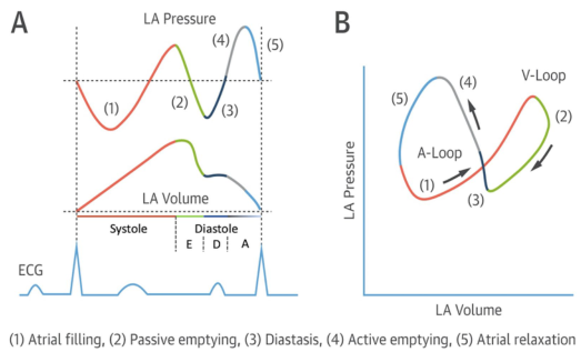
Summary : This figure illustrates the left atrial (LA) pressure-volume relationship during the cardiac cycle, showing both time-course traces and a pressure-volume loop, with key phases of atrial function annotated and correlated with the ECG. line plot and loop diagram: # Panel A: LA Pressure and Volume Traces • Top trace: LA Pressure (y-axis, arbitrary units) over time. • Middle trace: LA Volume (y-axis, arbitrary units) over time. • Bottom trace: ECG waveform for temporal reference. • X-axis: Cardiac cycle phases, with systole and diastole labeled; diastole further subdivided into E, D, and A phases. • Five phases are color-coded and numbered: – (1) Atrial filling (red) – (2) Passive emptying (green) – (3) Diastasis (black) – (4) Active emptying (blue) – (5) Atrial relaxation (gray) • Vertical dashed lines demarcate transitions between phases. # Panel B: LA Pressure-Volume Loop • X-axis: LA Volume (arbitrary units). • Y-axis: LA Pressure (arbitrary units). • The loop is traced in a counterclockwise direction, with arrows indicating the sequence. • The same five phases (1–5) are color-coded as in Panel A. • The loop is divided into two segments: A-Loop (phases 1, 3, 4, 5) and V-Loop (phase 2). # Design Encodings : • Distinct colors for each phase (red, green, black, blue, gray). • Arrows on the loop indicate the direction of the cardiac cycle. • ECG trace provides timing reference for the pressure and volume changes. # Analysis : • The LA pressure and volume traces show cyclical changes corresponding to atrial filling, emptying, and relaxation. • The pressure-volume loop visually summarizes the dynamic relationship between LA pressure and volume, with distinct segments for passive and active phases. • The figure highlights the temporal coordination between atrial events and the ECG, emphasizing the mechanical and electrical coupling in the cardiac cycle.
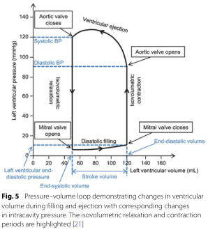
Summary : This figure shows a pressure–volume loop for the left ventricle, illustrating how ventricular volume and pressure change during the cardiac cycle, with key phases and valve events annotated. The isovolumetric relaxation and contraction periods are highlighted, and systolic/diastolic blood pressures are marked. pressure–volume loop diagram: # Title & Axes : • No explicit title on the figure, but the legend describes it as a "Pressure–volume loop demonstrating changes in ventricular volume during filling and ejection with corresponding changes in intracavity pressure." • X-axis: "Left ventricular volume (mL)" with tick marks at 0, 20, 40, 60, 80, 100, 120, 140, 160. • Y-axis: "Left ventricular pressure (mmHg)" with tick marks at 0, 20, 40, 60, 80, 100, 120, 140. • Additional axis labels: "Left ventricular end-diastolic pressure" (blue, left), "End-diastolic volume" (blue, bottom right), "Stroke volume" (black, bottom center). # Phases & Events : • Isovolumetric relaxation: vertical line at low volume, pressure drops, labeled. • Diastolic filling: horizontal line at low pressure, volume increases, labeled. • Isovolumetric contraction: vertical line at high volume, pressure rises, labeled. • Ventricular ejection: curved line, volume decreases as pressure peaks and falls, labeled. • Valve events: – Mitral valve opens (bottom left corner, low pressure/volume). – Mitral valve closes (bottom right corner, high volume/low pressure). – Aortic valve opens (top right corner, high volume/high pressure). – Aortic valve closes (top left corner, low volume/high pressure). # Blood Pressure Markers : • Systolic BP: horizontal dashed blue line at ~120 mmHg. • Diastolic BP: horizontal dashed blue line at ~80 mmHg. # Design Encodings : • Black solid lines for the loop. • Blue dashed lines for blood pressure markers. • Blue text for end-diastolic volume/pressure. • Labeled arrows for direction of phases and valve events. # Analysis : • The loop traces the cardiac cycle, starting at low pressure/volume (end-systolic), filling during diastole, rising sharply during isovolumetric contraction, ejecting blood during ventricular ejection, and dropping pressure during isovolumetric relaxation. • Systolic and diastolic blood pressures are marked, showing the pressure range during ejection. • The width of the loop (horizontal distance) represents stroke volume. • The figure clearly distinguishes the four main phases and the timing of valve openings/closings, providing a comprehensive view of ventricular mechanics during a heartbeat.
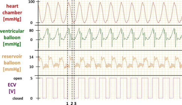
A multi-panel line graph illustrating the physiological mechanics of an in vitro cardiac loading device (CLD) used to simulate ventricular pressure-volume relationships. The visualization consists of four vertically aligned time-series plots depicting a cyclical cardiac simulator test. The top panel shows heart chamber pressure oscillating between 0 and 100 mmHg. The second panel displays ventricular balloon (VB) pressure, reaching peaks of approximately 80 mmHg. The third panel tracks reservoir balloon (RB) pressure, which fluctuates between 10 and 14 mmHg. The bottom panel indicates the status of an electronic check valve (ECV) as a binary voltage (0V for closed, 5V for open). Vertical dashed lines (labeled 1, 2, and 3) correlate specific phases: (1) ECV opening when VB pressure exceeds afterload, leading to VB emptying and RB filling; (2) VB refilling when VB pressure drops below RB pressure; and (3) ECV closure upon completion of refilling. This diagram is utilized in cardiovascular physiology research to validate cardiac cycle simulation for isolated heart preparations.
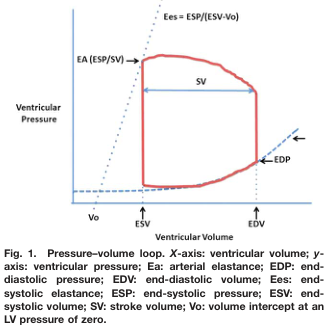
Summary : This figure presents a pressure–volume loop of the left ventricle, illustrating key cardiac parameters such as end-diastolic volume (EDV), end-systolic volume (ESV), stroke volume (SV), end-diastolic pressure (EDP), end-systolic pressure (ESP), arterial elastance (EA), and end-systolic elastance (Ees). The loop visually demonstrates the relationship between ventricular pressure and volume during a cardiac cycle. line plot: # Title & Axes : • Title: "Pressure–volume loop." • X-axis: "Ventricular Volume" (units not specified). – Tick labels: Vo (volume intercept at LV pressure of zero), ESV (end-systolic volume), EDV (end-diastolic volume). • Y-axis: "Ventricular Pressure" (units not specified). – No explicit tick labels shown. # Data & Curve : • Red closed loop traces the pressure–volume relationship during a cardiac cycle. • Horizontal arrow within the loop labeled "SV" (stroke volume) indicates the difference between EDV and ESV. • Vertical segments at EDV and ESV mark transitions between phases. • Dotted lines: – EA (arterial elastance) shown as a dashed line from Vo through ESP/SV. – Ees (end-systolic elastance) shown as a dashed line from Vo through ESP/(ESV-Vo). # Key Parameters & Annotations : • Vo: Volume intercept at LV pressure of zero (leftmost point on x-axis). • ESV: End-systolic volume (right vertical segment). • EDV: End-diastolic volume (far right on x-axis). • SV: Stroke volume (horizontal arrow between ESV and EDV). • EDP: End-diastolic pressure (arrow at bottom right of loop). • ESP: End-systolic pressure (top of loop). • EA: Arterial elastance (dashed line labeled EA (ESP/SV)). • Ees: End-systolic elastance (dashed line labeled Ees = ESP/(ESV-Vo)). # Design Encodings : • Red solid line for the pressure–volume loop. • Blue dashed lines for elastance relationships. • Arrows and labels for key parameters. • No gridlines or axis units specified. # Analysis : • The pressure–volume loop demonstrates the cardiac cycle phases, with the lower right corner representing end-diastole (high volume, low pressure) and the upper left corner representing end-systole (low volume, high pressure). • Stroke volume is visually indicated as the horizontal distance between EDV and ESV. • Elastance lines (EA and Ees) provide graphical representations of arterial and ventricular contractility. • The loop’s shape and annotations allow for assessment of cardiac function and mechanical properties.
cardiac axis ECG interpretation hexaxial
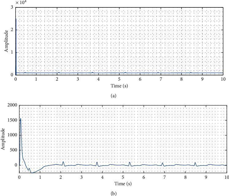
This Comparison Chart displays two waveform plots representing signal processing of an electrocardiogram (ECG) for cardiac arrhythmia diagnosis. Figure (a) illustrates the 'Raw signal' on a 10-second time axis with a high-amplitude y-axis scaled to 10^4. The raw data shows a significant initial artifact/spike reaching 3 x 10^4, which compresses the physiological cardiac waveforms. Figure (b) illustrates the 'Filtered signal' after noise reduction and intermediate filtration. The y-axis in the filtered view is adjusted to a range of -200 to 2000, allowing for the clear visualization of repetitive physiological ECG complexes that were previously obscured. Key educational concepts include signal-to-noise ratio improvement and the application of digital filters to physiological data for better clinical interpretation. This graphic is relevant for medical students and researchers studying diagnostic cardiology, signal processing in medicine, and automated arrhythmia detection systems.

This diagnostic image displays a single-lead electrocardiogram (ECG) trace plotted over a 15-second period, demonstrating the effects of cardiopulmonary resuscitation (CPR) on signal morphology. The x-axis represents time in seconds (0-15s) and the y-axis represents voltage in millivolts (mV). The trace is divided into two distinct pedagogical segments: a 10-second blue-highlighted block (0-10s) and a 5-second red-highlighted block (10-15s). The blue segment shows a high-frequency, high-amplitude waveform with significant mechanical artifacts and baseline instability characteristic of active chest compressions during CPR. These artifacts mask the underlying rhythm, showing oscillations between -1 mV and 1 mV. In contrast, the red segment (10-15s) illustrates a 'CPR pause' for pulse assessment. This section shows a much cleaner signal with a stable baseline and lower frequency, revealing distinct, organized QRS complexes. The image serves as a comparison chart for medical education, teaching the visual identification of CPR-related artifacts versus spontaneous cardiac rhythms and the necessity of pauses for accurate rhythm interpretation.
![This Comparison Chart illustrates simultaneous cardiac recordings using two different diagnostic modalities: Electrocardiography (ECG, top panel) and Magnetocardiography (MCG, bottom panel). The X-axis represents the number of samples (time progression), while the Y-axis indicates signal amplitude in arbitrary units [a.u.]. The ECG recording (blue trace) displays standard cardiac morphology, including identifiable P-waves, QRS complexes marked by green triangles, and T-waves. The MCG recording (orange trace) shows corresponding magnetic field fluctuations with peaks marked by red triangles. A significant feature of this graphic is the presence of high-amplitude noise and motion artifacts between samples 2500 and 5000, which disrupt the ECG signal more severely than the MCG. The image demonstrates the temporal synchronization between electrical and magnetic cardiac signals and the varying susceptibility of each modality to signal interference. This comparison is clinically relevant for evaluating the robustness of MCG as a complementary non-invasive tool for cardiac monitoring in high-interference environments.](https://cdn.orris.care/cdss_images/pmc_clinical_VQA_8ba087b002e9e100c9aad75ce6a81ac1e5a738e974e68f737cbe7a89029bf94f.jpg)
This Comparison Chart illustrates simultaneous cardiac recordings using two different diagnostic modalities: Electrocardiography (ECG, top panel) and Magnetocardiography (MCG, bottom panel). The X-axis represents the number of samples (time progression), while the Y-axis indicates signal amplitude in arbitrary units [a.u.]. The ECG recording (blue trace) displays standard cardiac morphology, including identifiable P-waves, QRS complexes marked by green triangles, and T-waves. The MCG recording (orange trace) shows corresponding magnetic field fluctuations with peaks marked by red triangles. A significant feature of this graphic is the presence of high-amplitude noise and motion artifacts between samples 2500 and 5000, which disrupt the ECG signal more severely than the MCG. The image demonstrates the temporal synchronization between electrical and magnetic cardiac signals and the varying susceptibility of each modality to signal interference. This comparison is clinically relevant for evaluating the robustness of MCG as a complementary non-invasive tool for cardiac monitoring in high-interference environments.
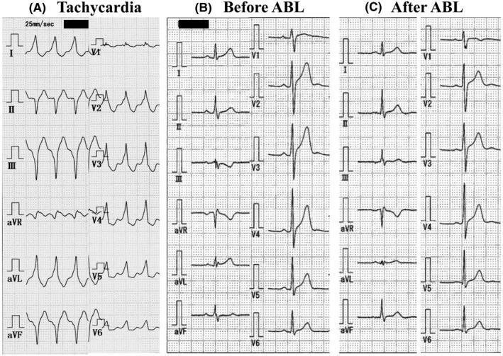
This diagnostic image displays three 12-lead electrocardiograms (ECGs) from a 33-year-old patient, comparing cardiac activity during tachycardia and sinus rhythm before and after catheter ablation. Panel (A) shows a wide QRS complex tachycardia characterized by a superior axis and positive concordance across the precordial leads (V1-V6). Panel (B) demonstrates a baseline 12-lead ECG in sinus rhythm before the procedure, showing no evidence of ventricular pre-excitation (no delta waves). Panel (C) captures the ECG following catheter ablation (ABL) of a Mahaim fiber. Key post-procedural changes include a significant increase in the R-wave amplitude in lead III and a rightward QRS axis shift from 12° to 59°. The comparison highlights subtle ECG indicators of successful ablation in cases of Mahaim-type accessory pathways where pre-excitation is not visible during normal sinus rhythm. This material is used to teach electrophysiological mapping and the interpretation of axis changes in supraventricular tachycardia management.
ECG axis deviation normal left right hexaxial reference system
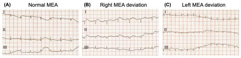
This diagnostic image displays a three-panel comparison of electrocardiogram (ECG) tracings illustrating Mean Electrical Axis (MEA) deviations in a small mammal model (O. degus). Each panel (A, B, C) presents standard bipolar leads I, II, and III on a red-grid background with a calibration of 50 mm/s and 20 mm/mV. (A) Normal MEA: Shows predominantly positive QRS complexes across leads I, II, and III, indicating a balanced electrical vector. (B) Right MEA Deviation: Characterized by a predominantly negative or smaller amplitude QRS deflection in lead I and a prominent positive deflection in lead III, signifying a rightward shift. (C) Left MEA Deviation: Demonstrates a strongly positive QRS deflection in lead I paired with a negative or small amplitude deflection in lead III, indicating a leftward shift. The tracings provide a visual reference for vector analysis and the diagnosis of cardiac axis shifts, highlighting morphology changes in the QRS complex, P waves, and T waves relevant to veterinary and comparative cardiology.
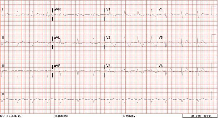
A standard 12-lead electrocardiogram (ECG) printed on red grid paper at 25 mm/sec. The tracing shows a normal sinus rhythm with a regular rate. Key conduction abnormalities are evident: a Right Bundle Branch Block (RBBB) is demonstrated by widened QRS complexes with a classic rSR' pattern and T-wave inversion in the right precordial leads (V1-V3), along with slurred S waves in leads I and V6. There is an associated Left Axis Deviation (LAD), suggested by the predominantly negative QRS complexes in leads II, III, and aVF, which may indicate a concomitant left anterior fascicular block (bifascicular block pattern). There is no significant ST-segment elevation (no STEMI), although minor non-specific ST-segment depression is visible in the inferior leads. The QT interval appears within normal limits. This ECG is representative of common conduction system disease used in cardiology education to identify fascicular and bundle branch blocks.
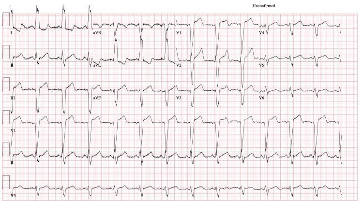
A 12-lead electrocardiogram (ECG) displayed on standard pink grid paper, demonstrating normal sinus rhythm with significant conduction abnormalities. The diagnostic hallmark is a Left Bundle Branch Block (LBBB), characterized by a markedly widened QRS complex exceeding 120ms (specifically 158ms per context). Notable morphology includes broad, notched, or 'M-shaped' R-waves in the lateral leads (I, aVL, V5, and V6) and deep S-waves in the right precordial leads (V1-V3). There is evidence of left axis deviation, with predominantly positive deflections in lead I and negative deflections in leads II and III. ST-segment and T-wave discordance is visible, where the ST-segments and T-waves shift in the opposite direction of the main QRS vector, a common secondary repolarization finding in LBBB. This diagnostic image is intended for medical education regarding cardiac conduction system delays and intraventricular blocks. The ventricular rate is approximately 78 bpm, and the QTc interval is prolonged at 533 ms.
The Cardiac Cycle - Simplified
The 7 Phases at a Glance
| Phase | ECG | Valves | Key Event | Heart Sound |
|---|---|---|---|---|
| A - Atrial Systole | P wave | Mitral OPEN | Atria contract, top up ventricle | S4 (if audible) |
| B - Isovolumetric Contraction | QRS | Mitral CLOSES | LV pressure rises, volume fixed | S1 (lub) |
| C - Rapid Ejection | ST segment | Aortic OPENS | Blood jets into aorta, LV volume falls fast | - |
| D - Reduced Ejection | T wave | Aortic still open | Ejection slows, aortic pressure starts to fall | - |
| E - Isovolumetric Relaxation | After T wave | Aortic CLOSES | LV pressure falls, volume fixed | S2 (dub) |
| F - Rapid Ventricular Filling | - | Mitral OPENS | LV fills passively from LA | S3 (if audible) |
| G - Reduced Ventricular Filling | - | Mitral open | Slow passive filling, diastasis | - |
Phase-by-Phase Explanation
A - Atrial Systole
- Triggered by the P wave (atrial depolarization)
- Atria contract → squeeze ~20% extra blood into already-filling ventricle
- Mitral valve is open; blood flows freely into LV
- The "a wave" appears on the venous pulse tracing
- S4 (4th heart sound): heard when the ventricle is stiff (e.g., LVH); atrium contracting against a non-compliant ventricle
B - Isovolumetric Contraction (IVC)
- Triggered by the QRS complex (ventricular depolarization)
- LV begins contracting → pressure rises sharply
- When LV pressure > LA pressure → mitral valve closes = S1 ("lub")
- All valves closed: LV pressure skyrockets, but volume does NOT change (isovolumetric)
- This is the most energy-intensive phase per unit time
C - Rapid Ventricular Ejection
- When LV pressure exceeds aortic pressure → aortic valve opens
- Blood is rapidly ejected into the aorta (~70% of stroke volume in this phase)
- LV volume falls sharply; aortic pressure rises to peak (~120 mmHg systolic)
- Corresponds to the ST segment
D - Reduced Ventricular Ejection
- Ventricles begin repolarizing → T wave begins
- Ejection continues but at a slower rate
- LV pressure starts to fall; blood "runs off" into arteries faster than ejection, so aortic pressure starts to fall
- LV volume reaches its minimum = End-Systolic Volume (ESV)
E - Isovolumetric Relaxation (IVR)
- After the T wave ends - LV fully repolarized and relaxed
- LV pressure falls below aortic pressure → aortic valve closes = S2 ("dub")
- All valves closed again: volume constant, pressure plummets
- The dicrotic notch (incisura) on the aortic pressure tracing marks valve closure
- Inspiration causes physiological splitting of S2 (pulmonic valve closes slightly later)
F - Rapid Ventricular Filling
- When LV pressure falls below LA pressure → mitral valve opens
- LV fills rapidly and passively (no active contraction)
- ~80% of ventricular filling happens passively here
- S3 (3rd heart sound): heard when ventricle is overfilled or dilated (e.g., heart failure, young normals) - "Ken-tuc-ky" rhythm
G - Reduced Ventricular Filling (Diastasis)
- Filling slows as pressure equilibrates between LA and LV
- The last slow trickle before the next P wave and atrial systole
Pressure-Volume Loop Summary
- Bottom right = end-diastole (EDV ~120 mL, low pressure)
- Top right corner = aortic valve opens
- Top left corner = aortic valve closes (end-systole, ESV ~50 mL)
- Stroke Volume = EDV - ESV = horizontal width of the loop
Key Numbers to Remember
| Parameter | Normal Value |
|---|---|
| Heart rate | 72 bpm |
| Cycle duration | ~0.833 sec |
| Systole | ~0.3 sec |
| Diastole | ~0.5 sec |
| EDV | ~120 mL |
| ESV | ~50 mL |
| Stroke Volume | ~70 mL |
| Ejection Fraction | ~60% |
At very fast heart rates, diastole shortens disproportionately - the ventricle doesn't fully fill before the next beat.
Cardiac Axis - Simple Interpretation
How It Works - The Concept
The Hexaxial Reference System
| Lead | Angle |
|---|---|
| Lead I | 0° |
| Lead II | +60° |
| Lead III | +120° |
| aVR | -150° |
| aVL | -30° |
| aVF | +90° |
Simple Quick Method - The "Lead I & aVF" Trick
         aVF positive?
              |
    YES       |       NO
     |         |        |
Lead I +  → NORMAL  Lead I + → LEFT axis deviation
Lead I -  → RIGHT   Lead I - → Extreme axis
| Lead I | aVF | Axis |
|---|---|---|
| Positive | Positive | NORMAL (0° to +90°) |
| Positive | Negative | LEFT axis deviation (-30° to -90°) |
| Negative | Positive | RIGHT axis deviation (+90° to +180°) |
| Negative | Negative | Extreme/Northwest axis (rare) |
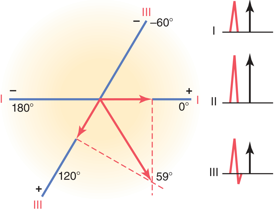
Axis Ranges - Defined
| Axis | Degrees | Category |
|---|---|---|
| -90° to -30° | Upper left | Left Axis Deviation (LAD) |
| -30° to +90° | Lower left-right | Normal |
| +90° to +180° | Lower right | Right Axis Deviation (RAD) |
| -90° to ±180° | Upper right | Extreme axis |
Why the Axis Deviates
Left Axis Deviation (LAD)
- Left ventricular hypertrophy (hypertension, aortic stenosis) - more LV muscle pulls vector left
- Left anterior fascicular block (LAFB) - most common cause of marked LAD
- Inferior MI - inferior wall scar, depolarization redirected superiorly
- LBBB - altered depolarization sequence
- Obese/pregnant patients (diaphragm pushes heart horizontally)
Right Axis Deviation (RAD)
- Right ventricular hypertrophy (cor pulmonale, pulmonary stenosis, tetralogy of Fallot)
- Left posterior fascicular block (LPFB)
- Right bundle branch block (RBBB)
- Normal in children and tall thin adults (vertical heart position)
- Deep inspiration (heart hangs more vertically)
Extreme Axis
- Hyperkalemia
- Ventricular tachycardia
- Emphysema (severe)
Quick Memory Aid
"Lead I and aVF are your best friends for axis."
- Both positive = Normal (thumbs up from both = happy)
- I positive, aVF negative = LAD (aVF unhappy = pulls LEFT)
- I negative, aVF positive = RAD (lead I unhappy = pushes RIGHT)
Clinical Correlation Summary
| Finding | Think of |
|---|---|
| LAD + wide QRS | LBBB or LAFB |
| RAD + tall R in V1 | RVH, RBBB |
| RAD in young child | Normal |
| Axis shift from old ECG | New fascicular block, new MI |
| Extreme axis | VT, hyperkalemia |