Dr Amandeep Singh, a cardiologist at a major teaching hospital, is reviewing a recently published cohort study that followed 50,000 adults for 15 years. The study found that people who drink 1-2 glasses of red wine daily have a 40% lower risk of heart disease compared to non-drinkers (RR=0.60, 95% CI: 0.45-0.80, p<0.001). The local media has picked up the story with headlines like "Red Wine: The Heart-Healthy Choice Doctors Recommend". However, Dr Singh notices some concerning patterns in the baseline characteristics table. Wine drinkers were more likely to be college-educated (78% vs 45%); have higher incomes (median £65,000 vs £35,000); exercise regularly (65% vs 32%); eat Mediterranean-style diets (71% vs 28%); and have regular healthcare check-ups (89% vs 54%). Non-drinkers included a higher proportion of former alcoholics (23%) and people with religious/cultural prohibitions against alcohol (31%). Dr Singh is now questioning whether red wine truly protects against heart disease or whether other factors might explain this association. I'd like the group to identify potential confounders in this scenario and explain your reasoning. What variables might be associated with both wine consumption and heart disease risk? Please bring evidence from your clinical experience to support your discussion of how these factors might operate. Let's explore the concept of confounding more deeply. Can you construct a simple diagram showing the relationships between wine consumption, the potential confounders you've identified, and heart disease outcomes? I want the group to consider: what makes a variable a true confounder versus just a risk factor? Now I'd like you to discuss what methods the researchers could have used at the design stage to control for these confounders. What are the advantages and limitations of each approach in this specific scenario? Please consider the practical implications for conducting such a study. Finally, let's consider the analysis stage. The authors reported they 'adjusted for age, sex, and smoking status'. Based on your confounding analysis, is this sufficient? What additional variables would you want to see included in a multivariable model, and why? I want the group to think about the concept of residual confounding – can we ever control for everything? The following article could help you: Hernán, M.A. and Robins, J.M. (2020) 'Confounding', in Causal Inference: What If. Boca Raton: Chapman & Hall/CRC, Chapter 7. Available at: https://static1.squarespace.com/static/675db8b0dd37046447128f5f/t/677676888e31cc50c2c33877/1735816881944/hernanrobins_WhatIf_2jan25.pdf

Reading File

Reading Web Page

confounding confounder definition adjustment control methods

Finding Sources

Searching PubMed

"alcohol" AND "cardiovascular disease" AND "confounding"

Finding Sources

Searching PubMed

"alcohol" AND "healthy user bias" AND "cardiovascular"

Reading Article

Reading File

Searching PubMed

"sick quitter" OR "abstainer bias" AND alcohol cardiovascular

Finding Sources

Searching PubMed

"Mendelian randomization" AND alcohol AND "cardiovascular disease"

Searching the Web

sick quitter bias abstainer bias alcohol cardiovascular studies healthy user bias evidence 2023 2024

Reading Article

Finding Sources

Generating Image

Here is a structured, seminar-style teaching analysis across all four questions Dr Singh has raised.

Confounding in Observational Research: The Red Wine & Heart Disease Case

PART 1 — Identifying the Potential Confounders

What Is a Confounder?

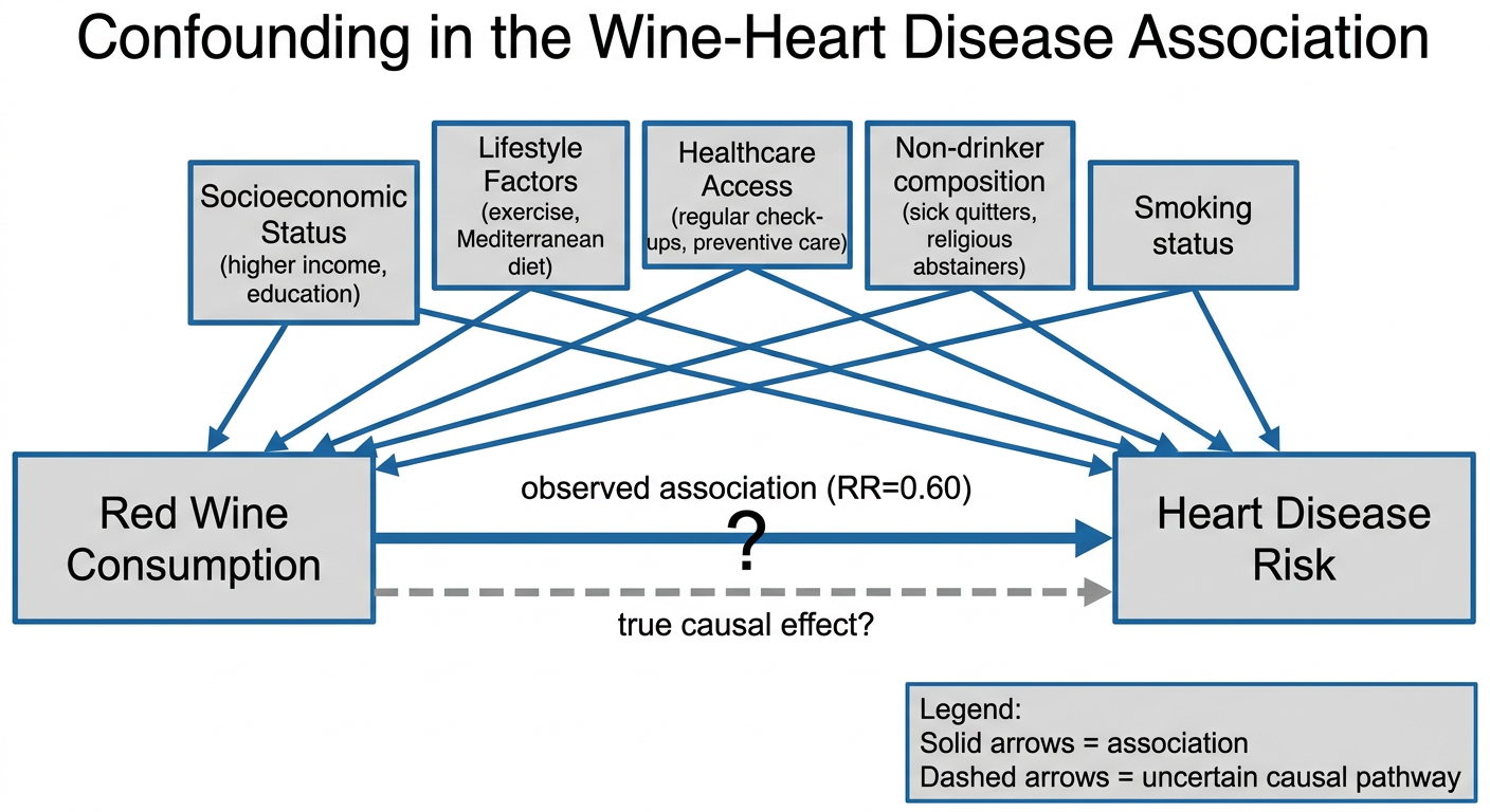
A confounder is a variable that is (1) associated with the exposure (wine drinking), (2) independently associated with the outcome (heart disease), and (3) not on the causal pathway between exposure and outcome — Goldman-Cecil Medicine defines it succinctly: "if a covariate is related to both the outcome and the exposure…and is unequally distributed between the groups being compared, it becomes a confounder." (Goldman-Cecil Medicine, 28th ed.)

Hernán & Robins frame this more rigorously using directed acyclic graphs (DAGs): confounding exists when there is an open "backdoor path" from exposure to outcome that runs through a common cause — a path that does not represent the true causal effect of interest (Causal Inference: What If, Chapter 7).

The Confounders in This Study

The baseline characteristics table reveals a highly unequal distribution of health-relevant variables. Each of the following satisfies all three criteria for confounding:

Variable	Associated with wine drinking?	Associated with heart disease?	Not on causal pathway?
Socioeconomic status (income, education)	Yes — 78% vs 45% college-educated; £65k vs £35k income	Yes — higher SES → better housing, nutrition, lower occupational stress, less financial strain	Yes
Regular exercise	Yes — 65% vs 32%	Yes — exercise reduces CV risk by 35–50% (reduces BP, improves lipid profiles, reduces insulin resistance)	Yes
Mediterranean diet	Yes — 71% vs 28%	Yes — strong independent protection against CVD (PREDIMED trial data)	Yes
Healthcare access	Yes — 89% vs 54% regular check-ups	Yes — earlier detection of hypertension, dyslipidaemia, diabetes	Yes
Smoking status	Likely — wine drinkers may have different smoking patterns	Yes — major independent CV risk factor	Yes
Non-drinker composition: "sick quitters"	Yes — 23% of non-drinkers are former alcoholics	Yes — former heavy drinkers have residual CV and hepatic damage	Not applicable (selection bias subtype)
Religious/cultural abstainers	Yes — 31% of non-drinkers	Varies — some cultural groups have higher/lower baseline CV risk	Not applicable

The "Sick Quitter" / "Abstainer Bias" Problem

This deserves special attention because it directly inflates the apparent benefit of drinking. By including former alcoholics (who quit due to illness) and never-drinkers with health-prohibitive conditions in the same "non-drinker" reference group, the comparator is systematically sicker. This is one of the most well-documented sources of bias in alcohol–cardiovascular studies.

A 2024 umbrella review (Sarich et al., Addiction) found that ~80% of mortality studies over the last 30 years failed to account for the sick-quitter effect, leading to systematic underestimation of alcohol-related harm. The Institute of Alcohol Studies summarises this clearly.

Confounder vs. Risk Factor: A Critical Distinction

Not every variable associated with the outcome is a confounder. To qualify, it must also be associated with the exposure and must not lie on the causal pathway. For example:

Age — if age is associated with both wine preference and heart disease and is not mediated by wine: confounder ✓
LDL cholesterol — if wine itself lowers LDL as part of its mechanism, adjusting for LDL would block the very causal pathway you're trying to study (this is an intermediate variable or mediator), and adjusting for it would introduce bias, not remove it. Hernán & Robins are explicit: "confounders cannot be descendants of treatment" — adjusting for intermediaries blocks causal paths and produces incorrect estimates.

PART 2 — Confounding Diagram (DAG)

Confounding in the Wine-Heart Disease Association

The diagram illustrates the core structural problem. Each confounder has arrows pointing to both wine consumption and heart disease risk — these are the "backdoor paths" that Hernán & Robins describe. The observed RR of 0.60 travels along the direct path and along every open backdoor path simultaneously. Until all backdoor paths are blocked (by adjustment), the estimated effect cannot be interpreted causally.

The sick-quitter/abstainer composition problem is distinct: it is better understood as selection bias in the reference group — the "non-drinker" category is not a clean unexposed group but a heterogeneous mixture of people with systematically worse health.

PART 3 — Design-Stage Methods to Control Confounding

A. Randomisation

What it does: Randomly assigns participants to wine vs. no-wine groups, distributing all confounders — known and unknown — equally between groups.

Advantages: The only method that controls for unmeasured confounders. No baseline differences in SES, diet, or exercise. As Miller's Anaesthesia notes: "Randomization distributes measured and unmeasured confounders evenly between groups." (Miller's Anaesthesia, 10e)

Limitations in this scenario:

Ethically problematic — you cannot randomise people to consume alcohol daily for 15 years
Practically impossible for a 15-year follow-up
Compliance issues: randomised participants may not adhere to assigned alcohol levels
Blinding is essentially impossible (participants know whether they're drinking wine)

B. Restriction

What it does: Restricts enrolment to a narrow, homogeneous subgroup (e.g., enrol only non-smokers with similar SES, or only moderate exercisers).

Advantages: Simple; eliminates confounding from the restricted variable entirely within the study population.

Limitations:

Severely limits generalisability (external validity)
Cannot restrict on all potential confounders simultaneously without making the study population impossibly small from 50,000 participants
Restricting on SES or lifestyle would make the sample unrepresentative of the general population

C. Matching

What it does: For each wine-drinking participant, identify a non-drinker matched on key confounders (age, sex, SES, smoking, exercise).

Advantages: Ensures distributional balance on matched variables; effective for a limited number of confounders; improves efficiency in case-control designs.

Limitations:

Difficult to match on more than 4–5 variables simultaneously
With 50,000 participants and many confounders (SES, diet, exercise, healthcare access, religion, prior alcohol history), many participants would be unmatchable and excluded, reducing power and introducing selection bias
Cannot match on unmeasured variables

D. Stratification at Design Stage

What it does: Pre-specify analysis within strata of confounders (e.g., analyse separately within high-SES and low-SES groups).

Limitations: With multiple confounders, sparse data in individual strata becomes a serious problem — the "curse of dimensionality."

Practical Recommendation for This Study

Given the scale (50,000 participants, 15 years), the most feasible design-stage intervention would have been prospective data collection with pre-specified measurement of all suspected confounders at baseline, combined with clear separation of the non-drinker reference group into lifetime abstainers vs. former drinkers vs. health-motivated abstainers. This addresses the sick-quitter problem at source.

PART 4 — Analysis-Stage Adjustment and Residual Confounding

Is Adjustment for Age, Sex, and Smoking Sufficient?

No — this is grossly insufficient. The study adjusted for three variables, but the baseline table reveals at least five major independent confounders that were left unadjusted:

Unadjusted Confounder	Why It Matters
SES (income + education)	Both independently predict heart disease through multiple pathways (diet, housing, stress, access to care)
Physical activity	65% vs 32% exercise rates — a massive imbalance with direct, strong CV protection
Mediterranean diet	71% vs 28% — PREDIMED data shows ~30% CV risk reduction independent of other factors
Healthcare utilisation	89% vs 54% — earlier hypertension and diabetes detection in wine drinkers
Non-drinker composition	Combining sick quitters (23%) and religious abstainers (31%) with healthy never-drinkers creates a biased reference group

The Mendelian randomisation data is instructive here. Biddinger et al. (2022, JAMA Network Open, PMID 35333364) used UK Biobank data (371,463 participants) and found that "light to moderate alcohol consumption was associated with healthier lifestyle factors, adjustment for which attenuated the cardioprotective epidemiological associations with modest intake." When they used genetic instruments to remove confounding, genetically predicted alcohol consumption was associated with increased cardiovascular risk, including a 1.4-fold higher risk of coronary artery disease. [PMID: 35333364]

Similarly, Larsson et al. (2020, Circ Genom Precis Med, PMID 32367730) using Mendelian randomisation found that genetically predicted higher alcohol consumption was associated with increased stroke and peripheral artery disease risk — directly contradicting the observational J-curve narrative. [PMID: 32367730]

The 2022 systematic review by Krittanawong et al. (Am J Med, PMID 35580715) across 1.58 million individuals in 56 cohorts concluded: "observational studies may overestimate the benefits of alcohol for cardiovascular disease outcomes… there are many confounding factors, in particular lifestyle, genetic, and socioeconomic associations with wine drinking, which likely explain much of the association." [PMID: 35580715]

What a Multivariable Model Should Include

A minimally adequate model for this study would need to adjust for:

Age and sex (already done)
Smoking (already done)
Physical activity (quantified — MET-hours/week)
Dietary pattern (Mediterranean diet score or fruit/vegetable intake)
SES composite (income + education as separate terms or an index)
Healthcare access (frequency of GP visits, insurance status)
Non-drinker subtype (lifetime abstainer vs. former drinker vs. health-restricted) — this is not adjustment but rather reference group redefinition
Comorbidities at baseline (BMI, pre-existing hypertension, diabetes, dyslipidaemia)
Social support / marital status (independent CV predictors often correlated with moderate drinking)

The Concept of Residual Confounding

Even with all of the above adjustments, residual confounding will remain. This is unavoidable in observational epidemiology for several reasons:

Measurement error in covariates — SES measured at a single point misses lifetime trajectory; diet questionnaires are imprecise; exercise is self-reported. Imperfect measurement of a confounder means imperfect adjustment.
Unknown and unmeasured confounders — We cannot adjust for what we have not measured. Genetic predispositions (e.g., ALDH2 variants affecting alcohol metabolism), personality traits, social network quality, and childhood exposures may all confound the relationship.
Time-varying confounding — Confounders may change over 15 years. Someone who starts exercising at year 5 and starts wine drinking at year 3 creates time-dependent confounding that standard regression cannot handle.
Granularity of adjustment — Adjusting for "exercise" as a binary yes/no is far less effective than a continuous quantitative measure. Coarse categorisation leaves within-category confounding.

Goldman-Cecil Medicine states this precisely: "All techniques to reduce confounding depend entirely on data about relevant covariates. If such data are missing, statistical adjustment cannot produce an accurate result." (Goldman-Cecil Medicine, 28th ed.)

Hernán & Robins formalise this under the concept of conditional exchangeability: the causal effect is identifiable only when, within levels of the measured covariates L, the treated and untreated groups are exchangeable (i.e., have the same potential outcomes). If unmeasured confounders U exist, this assumption fails.

Advanced Analysis Approaches Available

Method	Advantage	Limitation
Multivariable regression	Simple, interpretable	Cannot handle unmeasured confounders
Propensity score matching/weighting	Balances many confounders simultaneously; intuitive	Still only adjusts for measured variables
Instrumental variable analysis	Can address unmeasured confounding if a valid instrument exists	Valid instruments for alcohol consumption are rare; alcohol-related genetic SNPs (e.g., ADH1B, ALDH2) can serve as instruments in Mendelian randomisation
Mendelian randomisation	Uses genetic variants as "natural experiments"; randomises at conception so unmeasured lifestyle confounders are not inherited	Assumes genetic variant affects outcome only through the exposure (exclusion restriction); pleiotropy is a concern
Difference-in-differences	Can adjust for unmeasured time-stable confounders	Requires pre/post data; strong assumptions about parallel trends
Negative control outcomes	Tests whether the exposure affects an outcome with no plausible biological mechanism (if it does, confounding is present)	Requires identifying a credible negative control

Summary for Dr Singh's Group

The observed RR of 0.60 almost certainly overestimates any true cardioprotective effect of red wine. The confounding architecture in this study is severe:

Wine drinkers are systematically healthier, wealthier, better educated, more physically active, better fed, and better engaged with healthcare
The non-drinker reference group is diluted with former alcoholics and health-restricted abstainers who are systematically sicker
Adjustment for only age, sex, and smoking leaves the vast majority of confounding uncorrected
When Mendelian randomisation is used to approximate an unconfounded estimate, the apparent cardioprotective effect disappears and in some analyses reverses

The media headline "Red Wine: The Heart-Healthy Choice Doctors Recommend" is epidemiologically indefensible from this study. Dr Singh would be right to counsel that the association reflects the healthy wine-drinker rather than the wine that makes drinkers healthy.

The deeper lesson Hernán & Robins draw from Chapter 7 is conceptually important: confounding is not simply a statistical nuisance but a structural feature of the data-generating process. It cannot be fully resolved through analysis alone when the study design did not randomise exposure — residual confounding is the permanent epistemic ceiling of observational epidemiology.

Key References

Goldman-Cecil Medicine, 28th ed. (confounding, multivariable statistics)
Miller's Anaesthesia, 10e (confounding in research design)
Hernán MA & Robins JM (2020). Causal Inference: What If, Chapter 7 — confounding, DAGs, backdoor paths, conditional exchangeability
Krittanawong C et al. (2022). Alcohol Consumption and Cardiovascular Health. Am J Med. [PMID: 35580715]
Biddinger KJ et al. (2022). Association of Habitual Alcohol Intake With Risk of Cardiovascular Disease. JAMA Netw Open. [PMID: 35333364]
Larsson SC et al. (2020). Alcohol Consumption and Cardiovascular Disease: A Mendelian Randomization Study. Circ Genom Precis Med. [PMID: 32367730]

This is a shared conversation. Sign in to Orris to start your own chat.