
Biomarkers
What aspect of biomarkers are you interested in? · What's your goal?
biomarkers definition types classification overview 2025
biomarker types classification diagram overview
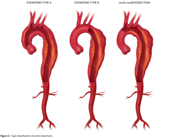
Summary : This figure illustrates the type classification of aortic dissections according to the Stanford system, showing three anatomical variants: Stanford Type A, Stanford Type B, and nonA-nonB dissection, with clear visualizations of the affected aortic segments. illustration: # Aortic Dissection Types : • Three labeled anatomical diagrams of the aorta, each showing a different type of aortic dissection. • Labels above each aorta: "STANFORD TYPE A", "STANFORD TYPE B", and "nonA-nonB DISSECTION". ## Stanford Type A : • Dissection involves the ascending aorta and extends beyond the aortic arch. • The false lumen (depicted as a split in the aortic wall) is present from the ascending aorta through the arch and into the descending aorta. ## Stanford Type B : • Dissection starts distal to the left subclavian artery, involving only the descending aorta. • The ascending aorta and arch are not involved. ## nonA-nonB Dissection : • Dissection involves the aortic arch but does not extend into the ascending aorta. • The false lumen is present in the arch and descending aorta, sparing the ascending aorta. # Scene Overview : • All diagrams are oriented with the aortic root at the top and the abdominal aorta at the bottom. • The aortic branches (brachiocephalic, left common carotid, left subclavian) are visible at the top of each diagram. • The false lumen is shown as a darker inner channel within the aortic wall. # Technical Details : • No scale bar or magnification is provided. • The diagrams use red and orange hues to differentiate the true and false lumens. # Spatial Relationships : • The three diagrams are aligned side-by-side for direct comparison. • The extent and location of the dissection vary between the types, highlighting the anatomical differences. # Analysis : • The figure visually distinguishes the three main anatomical patterns of aortic dissection. • Stanford Type A involves the ascending aorta, Stanford Type B is limited to the descending aorta, and nonA-nonB involves the arch without the ascending aorta. • This classification is critical for clinical decision-making and management of aortic dissections.
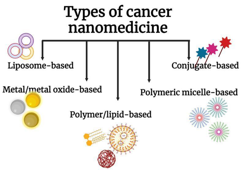
An educational infographic titled 'Types of cancer nanomedicine' providing a categorical classification of drug delivery systems. The diagram is organized hierarchically, branching into five primary categories of nanoparticles: 1) Liposome-based, illustrated as bilayered spherical vesicles; 2) Metal/metal oxide-based, depicted as solid inorganic spheres (e.g., gold or iron oxide); 3) Polymer/lipid-based, showing complex structures including lipid bilayers and polymer chains; 4) Polymeric micelle-based, represented as amphiphilic starburst arrangements with hydrophobic cores and hydrophilic shells; and 5) Conjugate-based, shown as small molecules attached to targeting ligands or polymers. The visual provides a fundamental overview of nanotechnology applied to oncology, focusing on diverse vehicle morphologies used to enhance drug solubility, prolong circulation, and improve targeted delivery to tumor sites. This classification is essential for understanding the pharmacological differences between approved nanodrugs and those in clinical development.
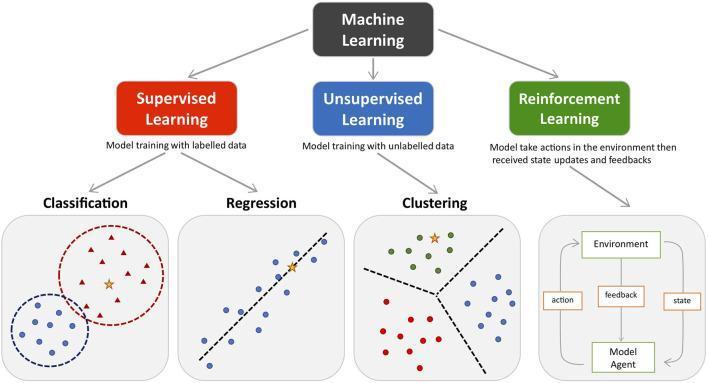
Educational flowchart and conceptual diagram illustrating the three primary domains of machine learning (ML) applicable to precision medicine, clinical diagnostics, and biomarker identification. The top level categorizes ML into Supervised Learning (model training with labeled data), Unsupervised Learning (model training with unlabeled data), and Reinforcement Learning (iterative learning via environmental feedback). Under Supervised Learning, two sub-types are shown: 'Classification,' depicting data separated into discrete categories (red triangles vs. blue dots) with a decision boundary, and 'Regression,' showing a continuous relationship with a linear trend line. Under Unsupervised Learning, 'Clustering' demonstrates the grouping of ambiguous data into distinct clusters (red, green, and blue dots) without prior labels. Reinforcement Learning is represented by a feedback loop between a 'Model Agent' and its 'Environment' involving actions, states, and feedback. Yellow stars throughout the diagram represent new, incoming data points (e.g., a patient's clinical profile) being processed or predicted by the trained models. This visual serves as a foundational guide for understanding how AI is integrated into clinical research for patient stratification and therapeutic decision-making.
Biomarkers: Definition, Types, and Uses
What Is a Biomarker?
- Proteins, lipids, or metabolites in blood or urine
- Genomic or proteomic patterns
- Imaging findings (radiomics)
- Electrical signals (e.g., ECG patterns)
- Cells present in bodily fluids
- Epigenetic marks (e.g., methylation products)
The 7 Official FDA/NIH Categories (BEST Glossary)
| Category | What It Tells You | Example |
|---|---|---|
| Susceptibility / Risk | Identifies people at elevated risk before disease appears | BRCA1/2 mutations → breast cancer risk |
| Diagnostic | Detects or confirms a disease is present | Troponin T → myocardial infarction; PSA → prostate cancer |
| Prognostic | Predicts how the disease will progress / outcome | HER2 overexpression → more aggressive breast cancer |
| Predictive | Predicts whether a patient will respond to a specific treatment | PD-L1 expression → likely response to immunotherapy |
| Pharmacodynamic / Response | Shows that the body has responded to an intervention | Serial ctDNA levels falling after chemotherapy |
| Monitoring | Tracks disease over time or detects recurrence | PSA rise after prostatectomy signals recurrence |
| Safety | Signals drug-related toxicity | Creatinine / eGFR → kidney safety monitoring in trials |
These categories are not mutually exclusive - a single biomarker can serve multiple roles depending on context.
Types by Biological Source
| Type | Examples |
|---|---|
| Molecular / genomic | Mutations (BRCA, KRAS, EGFR), gene expression arrays |
| Proteomic | Troponin, BNP, CA-125, CEA, AFP |
| Metabolomic | Blood glucose, lactate, lipid panels |
| Cellular | Circulating tumor cells (CTCs), CD4 T-cell count |
| Imaging / radiologic | CT density (Hounsfield units), PET SUV, MRI signal patterns |
| Physiologic | Blood pressure, eGFR, spirometry |
| Epigenetic | DNA methylation patterns |
| Liquid biopsy | Circulating tumor DNA (ctDNA), exosomes, microRNA |
What Makes a Good Biomarker?
- Easily measurable - from blood, urine, or a simple scan
- Reproducible - gives the same result across labs and time points
- Sensitive and specific - correctly identifies disease presence/absence
- Cost-effective - practical for routine use
- Clinically interpretable - the result drives a clear decision
The Biomarker Development Pipeline
- Discovery - Compare diseased vs. healthy samples; identify 10-100 candidate proteins/genes
- Verification - Develop targeted assays; narrow to 5-20 candidates with pilot studies (hundreds of patients)
- Validation - Rigorously validate the assay on thousands of samples; establish sensitivity, specificity, PPV, NPV; potentially seek FDA approval
Clinical Uses at a Glance
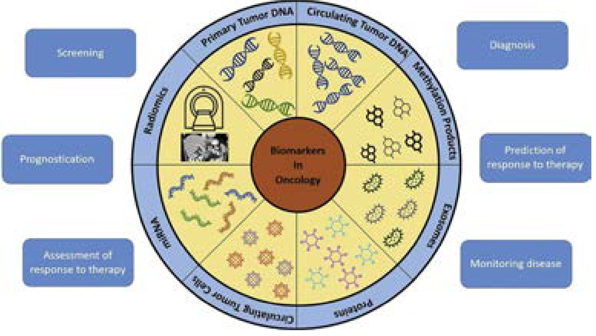
- Screening (e.g., PSA for prostate cancer)
- Diagnosis (e.g., stool ctDNA for colorectal cancer)
- Prognostication (e.g., BRCA1 mutation in breast cancer)
- Prediction of response (e.g., HER2 status for targeted therapy)
- Assessment of response (e.g., serial ctDNA monitoring)
- Early detection of recurrence (e.g., rising PSA post-surgery)
A Special Class: Surrogate Endpoint Biomarkers
The Frontier: Liquid Biopsy
- Brenner and Rector's The Kidney - Biomarker Definition chapter
- Tietz Textbook of Laboratory Medicine, 7th Ed. - Biomarker Pipeline chapter
- Current Surgical Therapy, 14th Ed. - Defining a Biomarker in oncology
- FDA BEST Glossary
- PMC - Biomarker definitions and their applications
How does a biomarker look like
troponin blood test cardiac biomarker
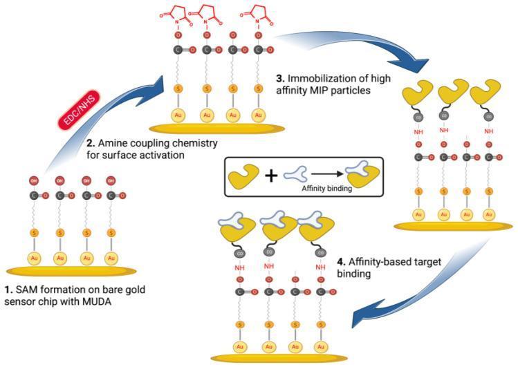
A technical four-step schematic illustrating the fabrication of a surface plasmon resonance (SPR) biosensor for cardiac Troponin I (cTnI) detection. Step 1: Formation of a self-assembled monolayer (SAM) of 11-mercaptoundecanoic acid (MUDA) on a bare gold (Au) sensor chip via sulfur (S) bonding. Step 2: Surface activation using EDC/NHS (N-ethyl-N'-(3-dimethylaminopropyl)carbodiimide/N-hydroxysuccinimide) amine coupling chemistry, showing the transition from carboxyl groups to activated NHS esters. Step 3: Immobilization of high-affinity molecularly imprinted polymer (MIP) particles, depicted as yellow crescent structures covalently attached to the surface. Step 4: Affinity-based target binding, where white irregularly shaped molecules (representing cTnI) bind specifically into the complementary cavities of the immobilized MIPs. This diagram demonstrates the principles of biomimetic sensor development, surface functionalization, and clinical biomarker detection for cardiovascular diagnostics.
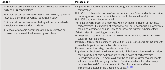
<table> <tr> <th>Grading</th> <th>Management</th> </tr> <tr> <td>G1: Abnormal cardiac biomarker testing without symptoms and with no ECG abnormalities</td> <td>All grades warrant workup and intervention, given the potential for cardiac compromise.<br> Hold ICPI for G1 elevated troponin<sup>a</sup> and recheck troponin 6 hours later. May consider resuming once normalized or if believed not to be related to ICPI.<br> Hold ICPI and discontinue for ≥ G2.</td> </tr> <tr> <td>G2: Abnormal cardiac biomarker testing with mild symptoms or new ECG abnormalities without conduction delay</td> <td>For patients with grade ≥ 2, early (ie, within 24 hours) initiation of high-dose corticosteroids (1-2 mg/kg/d of prednisone, oral or IV depending on symptoms) should be considered as it is likely to be beneficial without adverse effects.</td> </tr> <tr> <td>G3: Abnormal cardiac biomarker testing with either moderate symptoms or new conduction delay</td> <td>Admit patient for cardiology consultation.<br> Management of cardiac symptoms according to ACC/AHA guidelines and with guidance from cardiology.<br> Immediate transfer to a coronary care unit should be considered for patients with elevated troponin or conduction abnormalities.<br> For new conduction delay, consider a pacemaker.</td> </tr> <tr> <td>G4: Moderate to severe decompensation, IV medication or intervention required, life-threatening conditions</td> <td>In patients without an immediate response to high-dose corticosteroids, consider early institution of cardiac transplant rejection doses of corticosteroids (methylprednisolone 1 g every day) and the addition of either mycophenolate, infliximab, or antithymocyte globulin.<sup>210</sup> Consider abatacept (costimulatory molecule blockade) or alemtuzumab (CD52 blockade) as additional immunosuppression in life-threatening cases.<sup>211,212</sup></td> </tr> </table>
tumor marker CA-125 CEA protein structure lab test
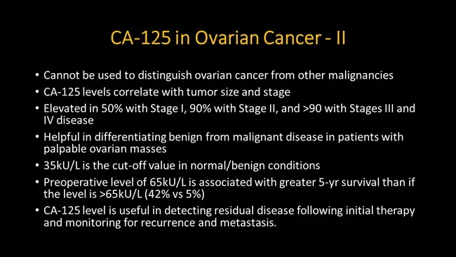
CA-125 in Ovarian Cancer — II This slide presents CA-125 as a biomarker for ovarian cancer in a text-based educational format rather than a radiologic image. The primary subject is CA-125 (MUC16), a serum biomarker whose levels correlate with tumor burden and stage in ovarian malignancy. Key points include that CA-125 elevation occurs in roughly half of patients with Stage I disease, about 90% of Stage II disease, and more than 90% with Stage III/IV disease. The slide notes a commonly used cut‑off around 35 kU/L for normal versus abnormal, and that a higher preoperative value (approximately 65 kU/L vs >65 kU/L) is associated with differential 5-year survival. Additional statements emphasize that CA-125 is useful for detecting residual disease after initial therapy and for monitoring recurrence and metastasis. The marker, however, cannot be used to distinguish ovarian cancer from other malignancies and may be elevated in benign gynecologic conditions or inflammatory states. Clinically, CA-125 informs staging, prognosis, treatment response, and surveillance and is typically interpreted alongside imaging and histopathology rather than as a standalone diagnostic test. The slide serves educational, research, and clinical practice purposes in gynecologic oncology and in studies of tumor biomarkers and longitudinal patient management.
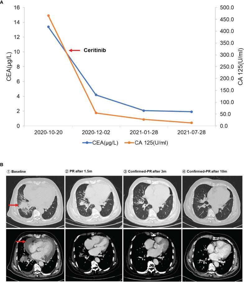
This composite educational graphic illustrates the longitudinal monitoring of a patient with ALK-positive non-small cell lung cancer (NSCLC) undergoing targeted therapy with ceritinib. Panel A is a line graph tracking serum tumor markers CEA (μg/L) and CA 125 (U/ml) over a nine-month period. It shows a rapid quantitative decline in both markers immediately following the initiation of ceritinib, which is marked by a red arrow. Panel B presents dynamic diagnostic imaging using axial CT scans at four intervals: Baseline, Partial Response (PR) after 1.5 months, Confirmed PR after 3 months, and Confirmed PR after 10 months. The lung window (top row) displays a right lung mass (red arrow) that significantly reduces in volume and density over time. The mediastinal window (bottom row) demonstrates a circumferential pericardial effusion (red arrow) at baseline that resolves nearly completely throughout the treatment course. This visual case study highlights the correlation between biochemical marker reduction and radiographic tumor regression (RECIST criteria) in oncological management.
circulating tumor DNA liquid biopsy diagram
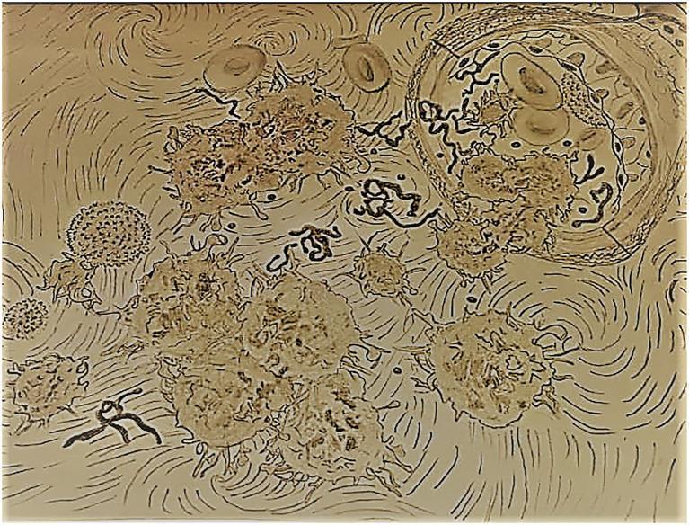
An educational medical illustration depicting the concept of liquid biopsy and circulating tumor components within the bloodstream. The diagram utilizes a stylized artistic rendering to show a cross-section of a blood vessel in the upper right corner, containing red blood cells and emerging tumor elements. Distributed throughout the swirling, fluid-like extracellular background are various 'tumor traces' targeted in oncology diagnostics: Circulating Tumor Cells (CTCs) shown as large, irregularly shaped clusters with prominent cytoplasmic projections; smaller, spherical circulating tumor exosomes; and fragmented, thread-like structures representing circulating tumor DNA (ctDNA) and RNA (ctRNA). The illustration serves to visualize the biological basis for liquid biopsy, emphasizing how genetic material and whole cells from a primary tumor enter systemic circulation, where they can be detected using molecular tools such as Next-Generation Sequencing (NGS) and PCR for cancer monitoring and personalized treatment.
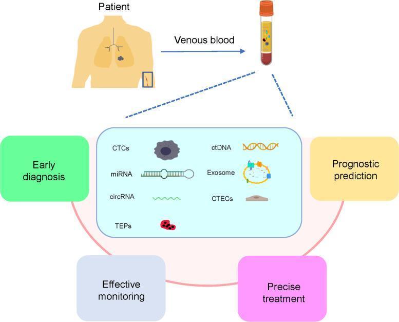
This medical infographic illustrates the clinical application of liquid biopsy in the management of lung cancer. The diagram depicts a patient with a primary lung tumor undergoing venous blood collection. The blood sample, shown in a collection tube, is analyzed for various circulating biomarkers. A central inset highlights seven key liquid biopsy components: circulating tumor cells (CTCs) as irregular dark cells; circulating tumor DNA (ctDNA) shown as double-helix strands; exosomes as membrane-bound vesicles; microRNAs (miRNA); circular RNAs (circRNA); tumor-educated platelets (TEPs); and circulating tumor vascular endothelial cells (CTECs). Four peripheral boxes describe the clinical utility of analyzing these biomarkers: early diagnosis, prognostic prediction, effective monitoring of disease progression, and precise treatment selection. This illustration serves as a summary of non-invasive diagnostic pathways, highlighting the role of liquid biopsy in capturing tumor heterogeneity and providing real-time clinical data for oncology.
What Does a Biomarker "Look Like"?
1. Molecules in the Blood (Proteins, DNA, RNA)
Liquid Biopsy Biomarkers (from a simple blood tube)
A patient gives a vial of blood. Inside that blood are multiple types of biomarkers: CTCs (circulating tumor cells - irregular dark cells), ctDNA (circulating tumor DNA - double-helix fragments), miRNA (short RNA strands), exosomes (tiny membrane bubbles), and circRNA. Each looks structurally different, even though they all come from the same blood sample.
2. Cells in the Bloodstream (Circulating Tumor Cells)
The large rough, clustered shapes are circulating tumor cells (CTCs). The thread-like fragments are ctDNA. The small round spheres are exosomes. Normal red blood cells (top right) are smooth, biconcave discs by comparison.
3. A Number on a Lab Report (Protein Biomarkers)
Panel A (top): The two lines show biomarker levels (CEA in blue, CA-125 in orange) falling rapidly after starting the drug ceritinib. This is what a "pharmacodynamic biomarker" looks like in practice - a falling number. Panel B (bottom): CT scans showing the tumor shrinking in parallel - confirming the biomarker was telling the truth.
4. An Imaging Signal (Radiologic Biomarker)
- A specific Hounsfield unit value on CT
- A PET scan hotspot (high glucose uptake = cancer)
- A particular MRI signal pattern
Summary Table
| Biomarker Type | What It Physically Looks Like |
|---|---|
| Protein (Troponin, PSA, CA-125) | A number in µg/L or U/mL on a lab report |
| Circulating tumor DNA (ctDNA) | Fragmented DNA double-helix strands in blood |
| Circulating Tumor Cells (CTCs) | Large, spiky, irregular cells under a microscope |
| Exosomes | Tiny membrane-bound spherical vesicles (nanoscale) |
| miRNA / circRNA | Short RNA strand sequences |
| Imaging biomarker | A brightness, density, or uptake pattern on a CT/PET/MRI |
| Genetic mutation (BRCA, EGFR) | A specific letter change in a DNA sequence |
How to do a biomarker project
What kind of biomarker project are you working on? · Where are you in the process?
how to plan a biomarker academic project steps methodology students
biomarker research study design pipeline workflow phases
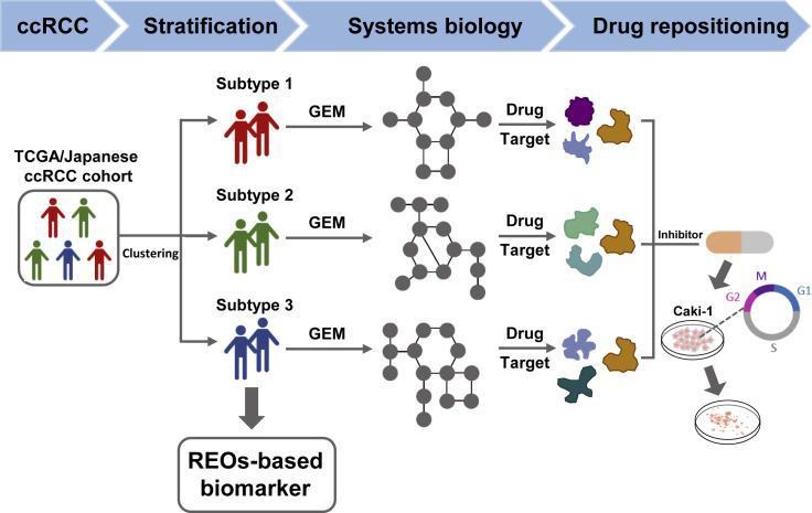
This medical flowchart illustrates a research pipeline for clear cell Renal Cell Carcinoma (ccRCC) study design, encompassing patient stratification, systems biology analysis, and drug repositioning. The workflow begins with a 'TCGA/Japanese ccRCC cohort' that undergoes 'Clustering' to stratify patients into three molecular subgroups: Subtype 1 (red), Subtype 2 (green), and Subtype 3 (blue). Parallel to this, a clinical 'REOs-based biomarker' is identified. In the 'Systems biology' phase, each subtype is processed through Genome-scale Metabolic Models (GEM), visually represented as distinct node-and-link networks. These models lead to 'Drug Target' identification, shown as diverse molecular shapes for each subtype. The 'Drug repositioning' phase focuses on an 'Inhibitor' (depicted as a therapeutic capsule) targeting these clusters. Experimental validation is shown using the Caki-1 cell line in petri dishes, demonstrating biological effects such as cell cycle arrest at the G2/M phase, indicated by a circular cell cycle diagram highlighting the transition from G2 to M. This flowchart maps the translation from multi-omic patient data to targeted therapeutic validation.
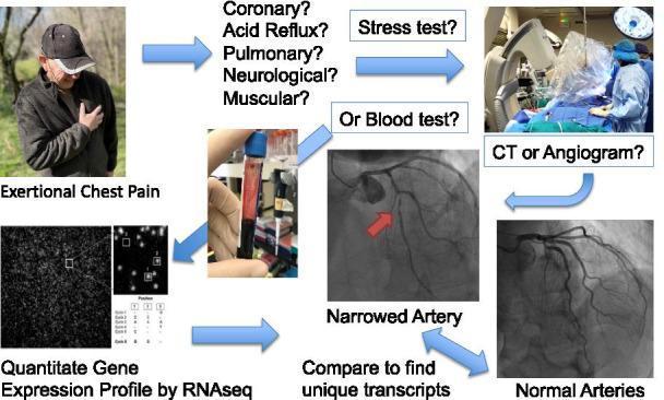
This scientific illustration and flowchart describe a clinical research study design evaluating blood-based RNA biomarkers for Coronary Artery Disease (CAD). The workflow begins with a clinical photograph of a patient experiencing exertional chest pain, prompting a differential diagnosis (Coronary, Acid Reflux, Pulmonary, Neurological, or Muscular). Diagnostic pathways shown include stress tests and blood tests, leading to imaging via CT or Angiogram. Radiological images illustrate the comparison between 'Normal Arteries' and a 'Narrowed Artery' (indicated by a red arrow). The research component is depicted through a photograph of a blood sample collection and a visualization of quantitative gene expression profiling via RNAseq. The final stages involve comparing transcriptomic data from 'LOW CAD' (<20% stenosis) and 'MID+ CAD' (>20% stenosis) groups to identify unique transcripts. The diagram effectively bridges clinical presentation, diagnostic imaging (angiography), and molecular biology techniques (RNA sequencing) to define a methodology for cardiovascular biomarker discovery.
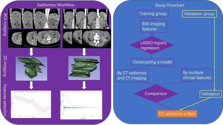
This infographic illustrates a dual-pane flowchart detailing a radiomics workflow and an associated clinical study design for oncology research. The left pane, titled 'Radiomics Workflow,' depicts the technical pipeline: starting with 'ROI imaging' showing segmented contrast-enhanced abdominal CT scans (coronal and axial views), followed by '2D imaging' which displays 3D reconstructions and surface renderings of tumor morphology, and concluding with 'Features selection' represented by LASSO regression plots and coefficient profiles. The right pane, 'Study Flowchart,' outlines the methodological framework: initial data is split into a 'Training group' and 'Validation group.' The training pipeline involves the extraction of 856 imaging features, dimensionality reduction via LASSO logistic regression, and the construction of comparative predictive models. These models compare 'CT radiomics and CT imaging' against 'multiple clinical features' (e.g., T stage, lymph vessel invasion). The final stage indicates a model 'Comparison' and subsequent 'Validation,' concluding that the CT radiomics approach demonstrates superior predictive performance for outcomes such as lymph node metastasis.
How to Do a Biomarker Academic Project (From Scratch)
Step 1 - Choose Your Topic and Research Question
- What disease or condition am I interested in? (e.g., diabetes, heart disease, cancer, kidney injury)
- What role should the biomarker play? (diagnosis, prognosis, monitoring, treatment response)
- Is there a gap in current knowledge? (e.g., "There is no reliable early biomarker for X")
- "Can troponin levels predict 30-day mortality in sepsis patients?"
- "Is PSA a reliable screening biomarker for prostate cancer in men under 50?"
- "Do blood glucose levels correlate with cognitive decline in Type 2 diabetes?"
Tip: Keep it narrow. "Biomarkers in cancer" is too broad. "CEA as a monitoring biomarker in colorectal cancer after surgery" is a workable project.
Step 2 - Define the Type of Biomarker You Will Study
| Category | Your Question Type |
|---|---|
| Diagnostic | Can biomarker X detect disease Y? |
| Prognostic | Does biomarker X predict how serious the disease will be? |
| Predictive | Does biomarker X predict response to treatment Z? |
| Monitoring | Does biomarker X track disease over time? |
| Risk/Susceptibility | Does biomarker X identify people at risk before disease starts? |
| Pharmacodynamic | Does biomarker X show the drug is working? |
| Safety | Does biomarker X signal drug toxicity? |
Step 3 - Do a Literature Review
- PubMed (free) - the gold standard for medical research
- Google Scholar
- Your university library databases
- Has this biomarker been studied before?
- What were the sensitivity and specificity values reported?
- What gaps or limitations did previous studies mention?
- What patient populations were included?
Step 4 - Design Your Study
Choose your study design:
| Design | When to Use | Example |
|---|---|---|
| Literature review / systematic review | No lab access; synthesize existing evidence | Review all studies on BNP in heart failure |
| Retrospective study | Use existing patient records or data | Compare troponin levels in ICU survivors vs. non-survivors |
| Cross-sectional study | One-time measurement across a group | Measure HbA1c in diabetic vs. non-diabetic adults |
| Case-control study | Compare cases (disease) vs. controls (healthy) | Blood IL-6 in sepsis patients vs. healthy volunteers |
| Prospective cohort | Follow patients over time | Monitor PSA every 6 months in prostate cancer patients |
For most school projects, a literature-based systematic review or a retrospective analysis using publicly available datasets is the most practical approach.
Step 5 - Identify Your Biomarker Characteristics (What to Measure)
| Metric | What It Means |
|---|---|
| Sensitivity | % of diseased patients the biomarker correctly identifies (true positive rate) |
| Specificity | % of healthy people correctly identified as disease-free (true negative rate) |
| PPV (Positive Predictive Value) | If the test is positive, how likely is the patient actually sick? |
| NPV (Negative Predictive Value) | If the test is negative, how likely is the patient actually healthy? |
| ROC curve / AUC | Overall accuracy of the biomarker across all thresholds (AUC of 1.0 = perfect) |
| Cut-off / threshold value | The specific level above/below which the test is positive |
- Easily measurable from blood or urine
- Reproducible across labs
- Sensitive AND specific
- Cost-effective
- Stable in its sample matrix
Step 6 - Collect or Source Your Data
Option A - Use Publicly Available Datasets (Recommended for school projects)
- GEO (Gene Expression Omnibus) - genomic/proteomic data: ncbi.nlm.nih.gov/geo
- TCGA (The Cancer Genome Atlas) - cancer biomarker data
- UK Biobank - large population health dataset
- PhysioNet - ICU patient data
Option B - Primary Data Collection (Lab or Hospital)
- Recruit participants (or use anonymized existing samples)
- Collect samples (blood, urine, tissue)
- Run your assay (ELISA, PCR, mass spectrometry, etc.)
- Record clinical annotations alongside each sample
Step 7 - Analyze Your Results
- ROC curve analysis - to determine the best cut-off and calculate AUC
- t-test / Mann-Whitney U - to compare biomarker levels between groups
- Logistic regression - to test if the biomarker predicts an outcome
- Kaplan-Meier curves - if tracking survival over time
- Spearman/Pearson correlation - if comparing two continuous variables
Step 8 - Write Up Your Project
| Section | What to Include |
|---|---|
| Abstract | 1 paragraph summary of question, methods, results, conclusion |
| Introduction | Background on the disease, why this biomarker matters, research gap |
| Literature Review | What is already known; cite at least 10-15 papers |
| Aims & Hypotheses | 1-3 clear, testable statements |
| Methods | Study design, patient selection criteria, how biomarker was measured, statistical plan |
| Results | Tables + graphs of sensitivity, specificity, AUC, ROC curves |
| Discussion | What your results mean, compare to existing studies, limitations |
| Conclusion | Answer your research question; suggest future work |
| References | APA or Vancouver style |
Quick Project Checklist
- Focused research question defined
- Biomarker type and role identified
- Literature review done (PubMed, Google Scholar)
- Study design chosen (review, retrospective, cross-sectional, etc.)
- Data source identified (public dataset or primary collection)
- Key metrics planned (sensitivity, specificity, AUC)
- Statistical method chosen
- Report structure outlined
- Brenner and Rector's The Kidney - 5-Phase Biomarker Discovery & Validation Framework
- Tietz Textbook of Laboratory Medicine, 7th Ed. - Biomarker Pipeline
- University of Sheffield - How to do a research project
- PubMed - Free medical literature database