ECG

Asking for Preferences

Reading File

Finding Sources

Reading File

Searching Images

ECG basic interpretation P wave QRS complex T wave

Reading File

Searching Images

ECG axis leads chest leads placement 12-lead

Reading File

Loading Image

Here is a comprehensive guide to basic ECG interpretation, drawn primarily from Harrison's Principles of Internal Medicine, 22nd Ed. (2025) and Braunwald's Heart Disease.

ECG Basic Interpretation

What Is an ECG?

The electrocardiogram (ECG) records the electrical activity of the heart from body surface electrodes. A standard 12-lead ECG uses:

6 limb leads: I, II, III (bipolar) + aVR, aVL, aVF (unipolar augmented)
6 precordial (chest) leads: V1–V6

Each lead "looks" at the heart from a different angle. Leads II, III, aVF face the inferior wall; I, aVL face the lateral wall; V1–V4 face the anterior wall.

The ECG Grid

Small box = 0.04 s (horizontal) / 0.1 mV (vertical)
Large box = 0.20 s (horizontal) / 0.5 mV (vertical)
Standard paper speed: 25 mm/s

Normal Waveforms

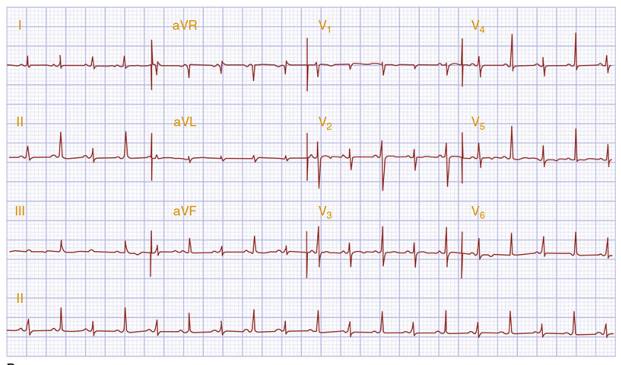
Normal sinus rhythm. Regular QRS complexes, narrow morphology, isoelectric ST segments, upright T waves in I, II, V2–V6.

Waveform	Represents	Normal
P wave	Atrial depolarization (SA node → AV node)	Duration < 0.12 s; amplitude < 2.5 mm; upright in I, II, aVF
PR interval	AV conduction time	0.12–0.20 s (3–5 small boxes)
QRS complex	Ventricular depolarization	Duration < 0.10–0.12 s; axis −30° to +100°
ST segment	Plateau of ventricular action potential	Isoelectric (no elevation or depression)
T wave	Ventricular repolarization	Upright in I, II, V2–V6; inverted in aVR (normal)
QT interval	Electrical systole	QTc ≤ 440 ms (men) / ≤ 460 ms (women)
U wave	Slow repolarization of His–Purkinje	Small, follows T wave (best seen V2–V3)

The Systematic Approach (Harrison's 14-Step Method)

A systematic approach prevents errors of omission. Analyze every ECG in this order:

Standardization / calibration — confirm 10 mm/mV calibration mark; check paper speed; identify artifacts and lead placement errors
Rhythm — regular vs. irregular; identify P waves; assess P–QRS relationship
Heart rate — count R–R intervals; 300 ÷ (# large boxes between R waves) for regular rhythms; or count complexes in 6 seconds × 10
PR interval — normal 0.12–0.20 s; prolonged = AV block; short = pre-excitation (WPW) or junctional rhythm
QRS interval — > 0.12 s = bundle branch block or ventricular rhythm
QT / QTc interval — prolonged QTc risks torsades de pointes
Mean QRS electrical axis — identify which lead has the most isoelectric (equiphasic) QRS; the axis is perpendicular to it
P waves — morphology (peaked = right atrial enlargement; notched/broad = left atrial enlargement)
QRS voltages — low voltage (< 5 mm in all limb leads) or high voltage (LVH criteria)
Precordial R-wave progression — R wave grows from V1 → V6; poor progression suggests anterior MI or LBBB
Abnormal Q waves — pathological Q wave = > 0.04 s wide and/or > 25% depth of following R wave; suggests prior MI
ST segments — elevation (injury/STEMI) vs. depression (ischemia/NSTEMI/reciprocal)
T waves — inversion (ischemia, strain, PE); hyperacute T waves (early STEMI); peaked/tall T waves (hyperkalemia)
U waves — prominent U waves suggest hypokalemia or drug effect (quinidine, amiodarone)

Always compare with any prior ECG — this is the single most valuable step.

Heart Rate Quick Calculation

For regular rhythms — count large boxes between two consecutive R waves:

Large boxes (R–R)	Rate (bpm)
1	300
2	150
3	100
4	75
5	60
6	50

Mnemonic: 300 – 150 – 100 – 75 – 60 – 50

QRS Axis

The frontal plane axis is assessed using limb leads:

Axis Range	Name	Causes
−30° to +100°	Normal	—
More negative than −30°	Left axis deviation (LAD)	Left anterior fascicular block, inferior MI, LBBB
More positive than +100°	Right axis deviation (RAD)	RVH, left posterior fascicular block, RBBB, PE
−90° to ±180°	Extreme axis	Ventricular tachycardia, lead reversal

Bedside trick: If lead I is positive (pointing left) and aVF is positive (pointing down) → normal axis. If I is positive and aVF is negative → suspect LAD; check if < −30° using lead II.

Ventricular Depolarization & R-Wave Progression

Ventricular depolarization has two major phases:

Septal depolarization — left → right → small r in V1, small q in V6
Free wall depolarization — dominated by LV mass → large S in V1, large R in V6

Normal R-wave progression: R amplitude increases progressively from V1 to V5/V6. The transition zone (R ≈ S) is normally V3 or V4.

Poor R-wave progression (small r waves persisting to V4–V5): suggests anterior MI, LBBB, or lead misplacement.

Key Intervals Summary

Interval	Normal	Abnormal
PR	0.12–0.20 s	Short: WPW, junctional; Long: 1st–3rd degree AV block
QRS	< 0.12 s	> 0.12 s: LBBB, RBBB, ventricular pacing/rhythm
QTc	≤ 440 ms ♂ / ≤ 460 ms ♀	Prolonged: drugs, electrolytes, congenital; Short: hypercalcemia

Normal ECG Example (12-lead)

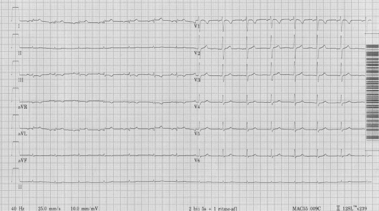
Regular sinus rhythm at ~60–75 bpm, narrow QRS, isoelectric ST segments, normal R-wave progression V1→V6, upright T waves.

Common Pitfalls

Lead reversal (RA–LA swap) mimics dextrocardia: global negativity in lead I, inverted P in I
Artifact can mimic arrhythmias (tremor → AF; movement → VT)
Left bundle branch block invalidates ST interpretation — always a "diagnostic challenge" per Harrison's
Computer interpretation has major limitations — clinician review is mandatory

Sources: Harrison's Principles of Internal Medicine, 22nd Ed. (2025), Chapter 247; Braunwald's Heart Disease, 12th Ed., Chapter 61.

Can I get altogether as a pdf file for future reference of opd

Reading File

Running Command

ls -la /home/daytona/workspace/

Running Command

mkdir -p /home/daytona/workspace/ecg-reference && ls /home/daytona/workspace/

Writing File

~/ecg-reference/generate_ecg_pdf.py

from reportlab.lib.pagesizes import A4
from reportlab.lib import colors
from reportlab.lib.styles import getSampleStyleSheet, ParagraphStyle
from reportlab.lib.units import cm, mm
from reportlab.platypus import (
    SimpleDocTemplate, Paragraph, Spacer, Table, TableStyle,
    HRFlowable, KeepTogether, Image as RLImage
)
from reportlab.lib.enums import TA_CENTER, TA_LEFT, TA_JUSTIFY
from reportlab.platypus import PageBreak
import urllib.request
import os

OUTPUT = "/home/daytona/workspace/ecg-reference/ECG_Basic_Interpretation_OPD_Reference.pdf"

# Download images
IMG_DIR = "/home/daytona/workspace/ecg-reference/imgs"
os.makedirs(IMG_DIR, exist_ok=True)

imgs = {
    "normal_ecg_12lead": "https://cdn.orris.care/cdss_images/HARRISON_1763035106721_34a37486-d246-47b9-a2dd-91a9c2d3da85.png",
    "normal_ecg_rhythm": "https://cdn.orris.care/cdss_images/pmc_clinical_VQA_8c1163b3750d607e08353561783f817d65e6286c06ce92932ad73574de25e590.jpg",
    "chest_leads": "https://cdn.orris.care/cdss_images/0a05159c6486e4e7ef48c4eb4c818c6727aa974175b9a8ad2c9d5531b49c5e5f.png",
    "ventricular_depol": "https://cdn.orris.care/cdss_images/3c19bed4b7dc721d6ff1f4789647829faec7c81d9446dec3cbcae6679dff7575.png",
}

downloaded = {}
for key, url in imgs.items():
    path = os.path.join(IMG_DIR, f"{key}.png")
    try:
        urllib.request.urlretrieve(url, path)
        downloaded[key] = path
        print(f"Downloaded: {key}")
    except Exception as e:
        print(f"Failed {key}: {e}")

# ── Styles ──────────────────────────────────────────────────────────────────
doc = SimpleDocTemplate(
    OUTPUT,
    pagesize=A4,
    leftMargin=1.8*cm, rightMargin=1.8*cm,
    topMargin=2*cm, bottomMargin=2*cm,
    title="ECG Basic Interpretation – OPD Quick Reference",
    author="Orris Medical Reference"
)

W = A4[0] - 3.6*cm   # usable width

styles = getSampleStyleSheet()

DARK_BLUE  = colors.HexColor("#1a3c5e")
MED_BLUE   = colors.HexColor("#2563a8")
LIGHT_BLUE = colors.HexColor("#dbeafe")
ACCENT     = colors.HexColor("#e8f4fd")
RED        = colors.HexColor("#c0392b")
ORANGE     = colors.HexColor("#d35400")
GREEN      = colors.HexColor("#1a7a4a")
GRAY       = colors.HexColor("#f5f7fa")
BORDER     = colors.HexColor("#b0c4de")

title_style = ParagraphStyle("Title2", parent=styles["Title"],
    textColor=DARK_BLUE, fontSize=22, spaceAfter=4, leading=28, alignment=TA_CENTER)

subtitle_style = ParagraphStyle("Subtitle", parent=styles["Normal"],
    textColor=MED_BLUE, fontSize=11, spaceAfter=2, alignment=TA_CENTER, leading=16)

h1_style = ParagraphStyle("H1", parent=styles["Heading1"],
    textColor=colors.white, fontSize=13, spaceBefore=10, spaceAfter=4,
    leading=18, backColor=DARK_BLUE, leftIndent=-4, rightIndent=-4,
    borderPadding=(4, 6, 4, 6))

h2_style = ParagraphStyle("H2", parent=styles["Heading2"],
    textColor=DARK_BLUE, fontSize=11, spaceBefore=8, spaceAfter=2,
    leading=15, borderPadding=(2, 0, 2, 0))

body_style = ParagraphStyle("Body", parent=styles["Normal"],
    fontSize=9.5, leading=14, spaceAfter=4, alignment=TA_JUSTIFY)

bullet_style = ParagraphStyle("Bullet", parent=styles["Normal"],
    fontSize=9.5, leading=14, leftIndent=14, bulletIndent=4, spaceAfter=2)

caption_style = ParagraphStyle("Caption", parent=styles["Normal"],
    fontSize=8, textColor=colors.HexColor("#555555"), leading=11,
    alignment=TA_CENTER, spaceAfter=6, italics=1)

footer_style = ParagraphStyle("Footer", parent=styles["Normal"],
    fontSize=7.5, textColor=colors.HexColor("#888888"), alignment=TA_CENTER)

def h1(txt):
    return Paragraph(f"&nbsp; {txt}", h1_style)

def h2(txt):
    return Paragraph(txt, h2_style)

def body(txt):
    return Paragraph(txt, body_style)

def bullet(txt):
    return Paragraph(f"• &nbsp;{txt}", bullet_style)

def sp(h=4):
    return Spacer(1, h)

def hr():
    return HRFlowable(width="100%", thickness=0.5, color=BORDER, spaceAfter=4)

def caption(txt):
    return Paragraph(f"<i>{txt}</i>", caption_style)

def table_style_base(header_bg=DARK_BLUE, row_alt=ACCENT):
    return TableStyle([
        ("BACKGROUND", (0,0), (-1,0), header_bg),
        ("TEXTCOLOR",  (0,0), (-1,0), colors.white),
        ("FONTNAME",   (0,0), (-1,0), "Helvetica-Bold"),
        ("FONTSIZE",   (0,0), (-1,0), 9),
        ("ROWBACKGROUNDS", (0,1), (-1,-1), [colors.white, row_alt]),
        ("FONTNAME",   (0,1), (-1,-1), "Helvetica"),
        ("FONTSIZE",   (0,1), (-1,-1), 9),
        ("GRID",       (0,0), (-1,-1), 0.4, BORDER),
        ("VALIGN",     (0,0), (-1,-1), "MIDDLE"),
        ("TOPPADDING", (0,0), (-1,-1), 4),
        ("BOTTOMPADDING", (0,0), (-1,-1), 4),
        ("LEFTPADDING",   (0,0), (-1,-1), 6),
        ("RIGHTPADDING",  (0,0), (-1,-1), 6),
        ("ALIGN",      (0,0), (-1,-1), "LEFT"),
    ])

# ── Build Story ─────────────────────────────────────────────────────────────
story = []

# ── HEADER ──
story.append(sp(6))
story.append(Paragraph("ECG Interpretation", title_style))
story.append(Paragraph("OPD Quick Reference Card", subtitle_style))
story.append(Paragraph("<font color='#888888' size='8'>Based on Harrison's Principles of Internal Medicine, 22nd Ed. (2025) &amp; Braunwald's Heart Disease</font>", caption_style))
story.append(sp(4))
story.append(hr())
story.append(sp(6))

# ── NORMAL 12-LEAD ECG IMAGE ──
if "normal_ecg_12lead" in downloaded:
    img = RLImage(downloaded["normal_ecg_12lead"], width=W, height=W*0.38)
    story.append(img)
    story.append(caption("Normal 12-lead ECG — sinus rhythm, narrow QRS, isoelectric ST, normal R-wave progression V1→V6"))
    story.append(sp(6))

# ── SECTION 1: THE GRID ──
story.append(h1("1. The ECG Grid"))
story.append(sp(4))

grid_data = [
    ["Parameter", "Small Box", "Large Box"],
    ["Time (horizontal)", "0.04 s", "0.20 s"],
    ["Voltage (vertical)", "0.1 mV", "0.5 mV"],
    ["Paper speed", "25 mm/s (standard)", "—"],
]
t = Table(grid_data, colWidths=[W*0.4, W*0.3, W*0.3])
t.setStyle(table_style_base())
story.append(t)
story.append(sp(6))

# ── SECTION 2: LEADS ──
story.append(h1("2. The 12 Leads"))
story.append(sp(4))
story.append(body("<b>Limb leads:</b> I, II, III (bipolar) + aVR, aVL, aVF (unipolar augmented) — assess the <b>frontal plane</b>"))
story.append(body("<b>Precordial (chest) leads:</b> V1–V6 — assess the <b>horizontal plane</b>"))
story.append(sp(4))

territory_data = [
    ["Territory", "Leads", "Artery (usually)"],
    ["Inferior",     "II, III, aVF",    "RCA (80%) / LCx (20%)"],
    ["Lateral",      "I, aVL, V5, V6",  "LCx / Diagonal"],
    ["Anterior",     "V1–V4",           "LAD"],
    ["Septal",       "V1–V2",           "LAD (septal perforators)"],
    ["Posterior",    "V7–V9 / tall R in V1–V2", "RCA / LCx"],
    ["Right ventricle", "V3R–V4R",      "RCA (proximal)"],
]
t = Table(territory_data, colWidths=[W*0.22, W*0.33, W*0.45])
t.setStyle(table_style_base())
story.append(t)

if "chest_leads" in downloaded:
    story.append(sp(6))
    img = RLImage(downloaded["chest_leads"], width=W*0.45, height=W*0.42)
    story.append(img)
    story.append(caption("Precordial lead positions V1–V6 (Harrison's Fig. 247-5)"))

story.append(sp(6))

# ── SECTION 3: NORMAL WAVEFORMS ──
story.append(h1("3. Normal Waveforms & Intervals"))
story.append(sp(4))

wave_data = [
    ["Waveform / Interval", "Represents", "Normal Values"],
    ["P wave",        "Atrial depolarization (SA→AV node)",         "Duration < 0.12 s; amplitude < 2.5 mm\nUpright in I, II, aVF; inverted in aVR"],
    ["PR interval",   "AV conduction time",                          "0.12 – 0.20 s (3–5 small boxes)"],
    ["QRS complex",   "Ventricular depolarization",                  "Duration < 0.10–0.12 s\nAxis: −30° to +100°"],
    ["ST segment",    "Plateau of ventricular action potential",      "Isoelectric (no elevation/depression)"],
    ["T wave",        "Ventricular repolarization",                   "Upright: I, II, V2–V6\nInverted (normal): aVR"],
    ["QT interval",   "Total electrical systole",                    "QTc ≤ 440 ms ♂  |  ≤ 460 ms ♀"],
    ["U wave",        "Slow repolarization of His–Purkinje",         "Small, after T wave; best in V2–V3"],
]
t = Table(wave_data, colWidths=[W*0.22, W*0.38, W*0.40])
t.setStyle(table_style_base())
# wrap text
for row in range(1, len(wave_data)):
    for col in range(3):
        pass
story.append(t)
story.append(sp(6))

# ── SECTION 4: 14-STEP SYSTEMATIC APPROACH ──
story.append(h1("4. Systematic Approach — Harrison's 14 Steps"))
story.append(sp(4))
story.append(body("A systematic approach prevents errors of omission. Analyze every ECG in this sequence:"))
story.append(sp(3))

steps = [
    ("1", "Standardization / calibration", "Confirm 10 mm/mV mark; check paper speed; look for artifacts & lead reversal"),
    ("2", "Rhythm", "Regular vs. irregular; identify P waves; assess P–QRS relationship"),
    ("3", "Heart rate", "300 ÷ (# large boxes between R waves) for regular rhythms; or count complexes in 6 s × 10"),
    ("4", "PR interval / AV conduction", "Normal 0.12–0.20 s. Short = WPW / junctional. Long = AV block"),
    ("5", "QRS interval", "> 0.12 s = bundle branch block or ventricular rhythm"),
    ("6", "QT / QTc", "Prolonged QTc → risk of torsades de pointes"),
    ("7", "Mean QRS electrical axis", "Identify most isoelectric limb lead; axis is perpendicular to it"),
    ("8", "P waves", "Peaked (≥ 2.5 mm) = RAE; Broad/notched = LAE"),
    ("9", "QRS voltages", "Low voltage (< 5 mm all limb leads) or high voltage (LVH criteria)"),
    ("10", "R-wave progression", "R grows V1→V5/V6; poor progression = anterior MI / LBBB / lead error"),
    ("11", "Abnormal Q waves", "Pathological: > 0.04 s wide AND/OR > 25% of R wave depth → prior MI"),
    ("12", "ST segments", "Elevation = injury/STEMI. Depression = ischemia/NSTEMI/reciprocal changes"),
    ("13", "T waves", "Inversion = ischemia, strain, PE. Hyperacute = early STEMI. Peaked = hyperkalemia"),
    ("14", "U waves", "Prominent = hypokalemia, quinidine, amiodarone"),
]

step_table_data = [["#", "Parameter", "Key Points"]] + [[s[0], s[1], s[2]] for s in steps]
t = Table(step_table_data, colWidths=[W*0.06, W*0.30, W*0.64])
t.setStyle(table_style_base())
t.setStyle(TableStyle([
    ("BACKGROUND", (0,0), (-1,0), DARK_BLUE),
    ("TEXTCOLOR",  (0,0), (-1,0), colors.white),
    ("FONTNAME",   (0,0), (-1,0), "Helvetica-Bold"),
    ("FONTSIZE",   (0,0), (-1,0), 9),
    ("ROWBACKGROUNDS", (0,1), (-1,-1), [colors.white, ACCENT]),
    ("FONTNAME",   (0,1), (-1,-1), "Helvetica"),
    ("FONTSIZE",   (0,1), (-1,-1), 8.5),
    ("GRID",       (0,0), (-1,-1), 0.4, BORDER),
    ("VALIGN",     (0,0), (-1,-1), "TOP"),
    ("TOPPADDING", (0,0), (-1,-1), 3),
    ("BOTTOMPADDING", (0,0), (-1,-1), 3),
    ("LEFTPADDING",   (0,0), (-1,-1), 5),
    ("RIGHTPADDING",  (0,0), (-1,-1), 5),
    ("ALIGN",      (0,0), (0,-1), "CENTER"),
    ("FONTNAME",   (0,1), (0,-1), "Helvetica-Bold"),
    ("TEXTCOLOR",  (0,1), (0,-1), DARK_BLUE),
]))
story.append(t)
story.append(sp(4))
story.append(body("<b>⚑ Always compare with prior ECGs — the single most valuable step.</b>"))
story.append(sp(6))

# ── SECTION 5: HEART RATE ──
story.append(h1("5. Heart Rate Quick Reference"))
story.append(sp(4))

hr_data = [
    ["Large Boxes (R–R)", "Rate (bpm)", "Large Boxes (R–R)", "Rate (bpm)"],
    ["1", "300", "4", "75"],
    ["2", "150", "5", "60"],
    ["3", "100", "6", "50"],
]
t = Table(hr_data, colWidths=[W*0.25, W*0.25, W*0.25, W*0.25])
t.setStyle(table_style_base())
story.append(t)
story.append(sp(3))
story.append(body("<b>Mnemonic:</b> 300 – 150 – 100 – 75 – 60 – 50"))
story.append(body("For <b>irregular rhythms</b>: count all QRS complexes in a 10-second strip × 6"))
story.append(sp(6))

# ── SECTION 6: QRS AXIS ──
story.append(h1("6. QRS Electrical Axis"))
story.append(sp(4))

axis_data = [
    ["Axis Range", "Diagnosis", "Common Causes"],
    ["−30° to +100°", "Normal", "—"],
    ["< −30°",         "Left Axis Deviation (LAD)",   "Left anterior fascicular block, inferior MI, LBBB, LVH"],
    ["> +100°",        "Right Axis Deviation (RAD)",   "RVH, left posterior fascicular block, RBBB, PE, lateral MI"],
    ["−90° to ±180°",  "Extreme (indeterminate) axis", "VT, lead reversal, severe RVH"],
]
t = Table(axis_data, colWidths=[W*0.22, W*0.28, W*0.50])
t.setStyle(table_style_base())
story.append(t)
story.append(sp(4))

axis_trick_data = [
    ["Lead I", "aVF", "Axis"],
    ["Positive (↑)", "Positive (↑)", "Normal (roughly −30° to +90°)"],
    ["Positive (↑)", "Negative (↓)", "LAD — check lead II; if also negative → LAD confirmed"],
    ["Negative (↓)", "Positive (↑)", "RAD"],
    ["Negative (↓)", "Negative (↓)", "Extreme axis / indeterminate"],
]
t = Table(axis_trick_data, colWidths=[W*0.2, W*0.2, W*0.6])
t.setStyle(table_style_base(header_bg=MED_BLUE))
story.append(t)
story.append(caption("Bedside axis quick-check using leads I and aVF"))
story.append(sp(6))

# ── SECTION 7: R-WAVE PROGRESSION ──
story.append(h1("7. Ventricular Depolarization & R-Wave Progression"))
story.append(sp(4))

if "ventricular_depol" in downloaded:
    img = RLImage(downloaded["ventricular_depol"], width=W*0.55, height=W*0.32)
    story.append(img)
    story.append(caption("Two phases of ventricular depolarization — septal (vector 1, left→right) and free-wall (vector 2, LV-dominant) (Harrison's Fig. 247-6)"))
    story.append(sp(4))

story.append(body("<b>Phase 1 — Septal:</b> Left → right → small r in V1, small q in V6"))
story.append(body("<b>Phase 2 — Free wall:</b> LV-dominant, leftward/posterior → large S in V1, large R in V6"))
story.append(sp(3))
story.append(body("<b>Normal transition zone:</b> V3 or V4 (R ≈ S amplitude)"))

rwp_data = [
    ["Pattern", "Definition", "Causes"],
    ["Normal progression",     "R grows steadily V1 → V5/V6", "—"],
    ["Poor R-wave progression", "Small r in V3–V4 or V4–V5", "Anterior MI, LBBB, LVH, lead misplacement"],
    ["Early transition",        "Transition before V3",        "Posterior MI, WPW type B, RVH"],
    ["Late transition",         "Transition after V4",         "Anterior MI, LBBB"],
]
t = Table(rwp_data, colWidths=[W*0.28, W*0.32, W*0.40])
t.setStyle(table_style_base())
story.append(sp(4))
story.append(t)
story.append(sp(6))

# ── SECTION 8: KEY INTERVALS ──
story.append(h1("8. Key Intervals — Normal & Abnormal"))
story.append(sp(4))

interval_data = [
    ["Interval", "Normal", "Short — Think", "Prolonged — Think"],
    ["PR",     "0.12–0.20 s",               "WPW (delta wave), junctional rhythm",
     "1st-degree AV block (>0.20), 2nd/3rd-degree AV block"],
    ["QRS",    "< 0.10–0.12 s",             "—",
     "LBBB, RBBB, ventricular pacing/ectopy, hyperkalemia, Na-channel blockade"],
    ["QTc",    "≤ 440 ms ♂\n≤ 460 ms ♀",   "Hypercalcemia, digoxin, short QT syndrome",
     "Drugs (antiarrhythmics, antipsychotics, antibiotics), hypoK/Mg, congenital LQTS"],
]
t = Table(interval_data, colWidths=[W*0.10, W*0.17, W*0.33, W*0.40])
t.setStyle(table_style_base())
story.append(t)
story.append(sp(6))

# ── SECTION 9: COMMON PITFALLS ──
story.append(h1("9. Common Pitfalls & Caveats"))
story.append(sp(4))

pitfalls = [
    ("<b>Lead reversal (RA–LA swap):</b> Mimics dextrocardia — global negativity in lead I, inverted P in I; check electrode placement before interpreting"),
    ("<b>Artifact:</b> Muscle tremor mimics AF; patient movement mimics VT — always correlate clinically"),
    ("<b>LBBB:</b> Invalidates ST-segment interpretation for ischemia (new LBBB with chest pain = treat as STEMI equivalent per Sgarbossa criteria)"),
    ("<b>Rate-corrected QT (QTc):</b> Use Bazett formula — QTc = QT ÷ √(R–R in seconds). Inaccurate at very fast or slow rates"),
    ("<b>Computer interpretation:</b> Has major limitations — clinician review is mandatory before acting"),
    ("<b>Normal variants:</b> Early repolarization (J-point elevation in V2–V5 in young males); athletic bradycardia; incomplete RBBB"),
    ("<b>Posterior MI:</b> No direct ST elevation — look for tall R and ST depression in V1–V3 (mirror image); confirm with V7–V9"),
]
for p in pitfalls:
    story.append(bullet(p))
story.append(sp(6))

# ── SECTION 10: RHYTHM QUICK GUIDE ──
story.append(h1("10. Rhythm Quick Guide"))
story.append(sp(4))

rhythm_data = [
    ["Rhythm", "Rate", "P waves", "QRS", "Key Feature"],
    ["Normal sinus rhythm (NSR)", "60–100", "Upright in I, II, aVF before each QRS", "Narrow", "Regular R–R"],
    ["Sinus bradycardia",   "< 60",  "Normal", "Narrow", "Regular, slow"],
    ["Sinus tachycardia",   "> 100", "Normal", "Narrow", "Regular, fast; find cause"],
    ["Atrial fibrillation (AF)",   "Variable (100–160)", "No P waves; fibrillatory baseline", "Narrow (usually)", "Irregularly irregular"],
    ["Atrial flutter",      "Atrial ~300; ventricular varies", "Sawtooth flutter waves (II, III, aVF)", "Narrow", "Regular 2:1, 3:1, or 4:1 block"],
    ["SVT (AVNRT/AVRT)",    "150–250", "P buried in/after QRS or absent", "Narrow", "Abrupt onset/offset"],
    ["VT (ventricular tachycardia)", "> 100", "AV dissociation", "Wide (> 0.12 s)", "Fusion beats, capture beats"],
    ["VF (ventricular fibrillation)", "Rapid chaotic", "None", "Chaotic", "No organised QRS — code blue"],
    ["1st-degree AV block",  "Normal", "Normal (1:1)", "Narrow", "PR > 0.20 s"],
    ["2nd-degree AV block (Mobitz I)", "Normal/slow", "Progressive PR lengthening then dropped QRS", "Narrow", "Wenckebach — benign"],
    ["2nd-degree AV block (Mobitz II)", "Normal/slow", "Fixed PR, then sudden dropped QRS", "Often wide", "Risk of complete block"],
    ["3rd-degree AV block (CHB)", "Ventricular 30–50", "P waves and QRS dissociated", "Wide (escape)", "No relationship P→QRS"],
]
t = Table(rhythm_data, colWidths=[W*0.22, W*0.10, W*0.28, W*0.12, W*0.28])
t.setStyle(TableStyle([
    ("BACKGROUND", (0,0), (-1,0), DARK_BLUE),
    ("TEXTCOLOR",  (0,0), (-1,0), colors.white),
    ("FONTNAME",   (0,0), (-1,0), "Helvetica-Bold"),
    ("FONTSIZE",   (0,0), (-1,0), 8.5),
    ("ROWBACKGROUNDS", (0,1), (-1,-1), [colors.white, ACCENT]),
    ("FONTNAME",   (0,1), (-1,-1), "Helvetica"),
    ("FONTSIZE",   (0,1), (-1,-1), 8),
    ("GRID",       (0,0), (-1,-1), 0.4, BORDER),
    ("VALIGN",     (0,0), (-1,-1), "TOP"),
    ("TOPPADDING", (0,0), (-1,-1), 3),
    ("BOTTOMPADDING", (0,0), (-1,-1), 3),
    ("LEFTPADDING",   (0,0), (-1,-1), 4),
    ("RIGHTPADDING",  (0,0), (-1,-1), 4),
]))
story.append(t)
story.append(sp(6))

# ── SECTION 11: ISCHEMIA / STEMI LOCALIZATION ──
story.append(h1("11. ST-Elevation MI — Localization"))
story.append(sp(4))

stemi_data = [
    ["Location", "ST Elevation Leads", "Reciprocal Depression", "Culprit Artery"],
    ["Inferior",          "II, III, aVF",        "I, aVL",          "RCA (80%) / LCx"],
    ["Anterior",          "V1–V4",               "II, III, aVF",    "LAD (proximal)"],
    ["Anteroseptal",      "V1–V3",               "—",               "LAD"],
    ["Anterolateral",     "I, aVL, V3–V6",       "II, III, aVF",    "LAD / LCx diagonal"],
    ["Lateral",           "I, aVL, V5–V6",       "V1–V2",           "LCx / obtuse marginal"],
    ["Posterior",         "Tall R + ST↓ in V1–V3 (mirror)", "—",   "RCA / LCx"],
    ["Right ventricular", "V1, V4R (ST ↑ in V4R)", "—",            "RCA (proximal)"],
]
t = Table(stemi_data, colWidths=[W*0.20, W*0.22, W*0.22, W*0.36])
t.setStyle(table_style_base(header_bg=RED))
story.append(t)
story.append(sp(3))
story.append(body("<b>STEMI criteria (ESC/ACC/AHA):</b> ST elevation ≥ 1 mm in ≥ 2 contiguous limb leads OR ≥ 2 mm in ≥ 2 contiguous precordial leads, in the appropriate clinical context."))
story.append(sp(6))

# ── SECTION 12: BUNDLE BRANCH BLOCKS ──
story.append(h1("12. Bundle Branch Blocks"))
story.append(sp(4))

bbb_data = [
    ["Feature", "RBBB", "LBBB"],
    ["QRS duration", "> 0.12 s", "> 0.12 s"],
    ["V1 pattern",   "rSR' (M-shaped) / RSR'",    "Broad, deep QS or rS"],
    ["V6 pattern",   "Wide S wave",                "Broad, tall notched R (no Q)"],
    ["T wave",       "Inverted V1–V3 (secondary)", "Inverted I, aVL, V5–V6 (secondary)"],
    ["Axis",         "Usually normal",             "Usually LAD"],
    ["Ischemia assessment", "Possible but check cautiously", "LBBB invalidates ST analysis — use Sgarbossa"],
    ["Common causes", "RVH, PE, congenital, ischaemia", "Ischaemia, HTN, CMP, LBBB = always pathological"],
]
t = Table(bbb_data, colWidths=[W*0.28, W*0.36, W*0.36])
t.setStyle(table_style_base(header_bg=MED_BLUE))
story.append(t)
story.append(sp(6))

# ── SECTION 13: ELECTROLYTE EFFECTS ──
story.append(h1("13. Electrolyte Effects on ECG"))
story.append(sp(4))

elec_data = [
    ["Electrolyte", "Low (Hypo-)", "High (Hyper-)"],
    ["Potassium (K⁺)",
     "Flat/inverted T waves\nProminent U waves\nST depression\nProlonged QU",
     "Peaked (tall, narrow, symmetric) T waves\nPR prolongation → P wave disappears\nWide QRS → sine wave pattern (severe)\nVF risk"],
    ["Calcium (Ca²⁺)",
     "Prolonged QT (ST lengthening)\nT wave unchanged",
     "Short QT (short ST)\nT wave may steepen"],
    ["Magnesium (Mg²⁺)",
     "Prolonged PR, QRS, QT\nT wave flattening (often co-K⁺)",
     "Prolonged PR; rare ECG changes"],
    ["Sodium (Na⁺)",
     "Rare ECG changes",
     "Rare; severe hyperNa may widen QRS in Na-channel block context"],
]
t = Table(elec_data, colWidths=[W*0.20, W*0.40, W*0.40])
t.setStyle(table_style_base())
story.append(t)
story.append(sp(6))

# ── FOOTER NOTE ──
story.append(hr())
story.append(sp(4))
story.append(Paragraph(
    "This reference card is intended for educational purposes. Always correlate ECG findings with the full clinical picture. "
    "Generated by Orris Medical Reference | Sources: Harrison's Principles of Internal Medicine 22nd Ed. (2025); "
    "Braunwald's Heart Disease 12th Ed.",
    footer_style
))

# ── BUILD ────────────────────────────────────────────────────────────────────
doc.build(story)
print(f"\n✓ PDF saved to: {OUTPUT}")

Running Command

cd /home/daytona/workspace/ecg-reference && python generate_ecg_pdf.py

Your OPD reference PDF is ready! Here's the download link:

ECG Basic Interpretation OPD Reference

PDF Document · PDF

What's included in the PDF:

The ECG Grid — time & voltage values per box
The 12 Leads — territories, walls, and culprit arteries
Normal Waveforms & Intervals — P, PR, QRS, ST, T, QT, U with normal values
Harrison's 14-Step Systematic Approach — full table
Heart Rate Quick Reference — 300 rule mnemonic table
QRS Axis — normal/LAD/RAD with bedside I+aVF trick
Ventricular Depolarization & R-Wave Progression — with diagram
Key Intervals — PR, QRS, QTc with short/prolonged differentials
Common Pitfalls — lead reversal, artifact, LBBB, posterior MI
Rhythm Quick Guide — NSR through complete heart block
STEMI Localization — all territories with reciprocal leads
Bundle Branch Blocks — RBBB vs LBBB comparison
Electrolyte Effects — K, Ca, Mg on ECG

Includes 4 actual ECG images from Harrison's and clinical databases. Sourced from Harrison's 22nd Ed. (2025) and Braunwald's Heart Disease.

This is a shared conversation. Sign in to Orris to start your own chat.