
You are my personal professor, mentor, and High Performance Sports Scientist for the SAI Performance Analyst (Physiotherapy) examination. My examination is on 23 August. I have uploaded: 1. Official SAI Performance Analyst syllabus. 2. Official SAI exam scheme/reference document. These uploaded documents are the PRIMARY source for what must be covered. Use them as the roadmap. If you expand beyond them using textbooks or current sports science knowledge, clearly label that as additional context. Our objective is to COMPLETE the ENTIRE syllabus before the examination while maintaining conceptual clarity. IMPORTANT: Do NOT teach superficially. Do NOT give coaching-centre notes. Do NOT waste time on unnecessary details that are unlikely to help in the exam. Teach with the depth expected from postgraduate Sports Science while remaining focused on the SAI syllabus. Primary references should include: • McArdle, Katch & Katch – Exercise Physiology • ACSM Guidelines • NSCA Essentials of Strength & Conditio
python3 -c " from docx import Document doc = Document('/tmp/workspace/attachments/aea8320b-70ad-4b9d-8c28-9f787a098c55/SAI_Physiotherapy_Official_Syllabus_Reference-1.docx') for p in doc.paragraphs: style = p.style.name if p.style else 'None' if p.text.strip(): print(f'[{style}] {p.text}') "
SAI Performance Analyst (Physiotherapy) — Your Exam Command Centre
Exam Architecture — What You're Actually Fighting
| Section | Marks | Question Type | Your Strategy |
|---|---|---|---|
| A1 — Basic Sports Science (22 topics) | 32 | MCQ, interdisciplinary | Broad coverage, conceptual depth |
| A2 — General Sports Awareness | 8 | MCQ, factual | Rapid recall, current events |
| B — Applied Physiotherapy Knowledge | 40 | MCQ, discipline-specific | Deep clinical knowledge |
| C — Case Studies (Physiotherapy) | 20 | Passage-based, analytical | Clinical reasoning under time pressure |
Reading the Sample Questions — What SAI Actually Tests
18-Day Master Study Plan
Phase 1: Core Clinical Physiotherapy (Days 1–10) — 60 marks
| Day | Topic (Section B+C) | Priority Reason |
|---|---|---|
| 1–2 | Human Anatomy — Musculoskeletal focus (shoulder, knee, ankle, spine, hip) | Case studies are all musculoskeletal |
| 3 | Biomechanics — Gait analysis, joint biomechanics, sports-specific skills | B-section + C-section both test this |
| 4 | Sports Physiotherapy — Injury prevention, rehabilitation, screening, emergencies | Entire Section C is sports physio cases |
| 5 | Assessment & Clinical Reasoning — Special tests, Lachman, Hawkins-Kennedy, etc. | Every case study requires test knowledge |
| 6 | Exercise Therapy & Rehabilitation — PNF, progressive resistance, eccentric loading | Direct sample questions confirmed this |
| 7 | Electrotherapy — Modalities, TENS, ultrasound, LASER, IFT, SWD | B-section has direct electrotherapy questions |
| 8 | Exercise Physiology — Responses, adaptations, cardiorespiratory | Section A1 + Section B overlap |
| 9 | Sports Medicine, Nutrition & Research — Doping, basic nutrition, biostatistics | Section B + A overlap |
| 10 | Psychology & Human Development — Sport psych, growth & maturation | Section A1 topic 7 + Section B topic g |
Phase 2: Section A1 Consolidation (Days 11–15) — 32 marks
| Day | Topics |
|---|---|
| 11 | Anthropometry, Body Composition, Energy Systems, Fatigue |
| 12 | Strength & Conditioning principles, Load management, Periodization, Recovery protocols |
| 13 | Test parameters, Test protocols, Data interpretation, Performance profiling |
| 14 | Injury prevention & risk management, Technologies (GPS, IMU, wearables), Biostatistics |
| 15 | Yoga/mind-body, Anti-doping (WADA), Research methodology, Interdisciplinary coordination |
Phase 3: Section A2 + Revision + Mock Testing (Days 16–18) — 8 marks + Consolidation
| Day | Activity |
|---|---|
| 16 | General Sports Awareness — Olympics, Asian Games, Indian sports schemes, SAI governance |
| 17 | Full mock test (timed, 100 questions) using all sample questions + self-generated variants |
| 18 | Weak area targeted revision. No new topics. Mental preparation. |
How We Will Work Together
- Core Concepts — The mechanisms and principles you must own, not memorize
- Exam-Relevant Precision — Specific numbers, thresholds, classifications, and test names that appear in MCQs
- Clinical Reasoning Map — How to navigate Section C case vignettes for that topic
- Sample-Style Questions with Explanations — Matching the SAI question style
- High-Yield Summary — What to review the night before
Starting Point — Your Call
- Do you want to start with Day 1 (Musculoskeletal Anatomy) right now?
- Is there a specific topic you're weakest in that you want prioritized?
- Are you comfortable with the plan above, or do you want to adjust the sequence?
Start Day 1: Musculoskeletal Anatomy now
rotator cuff muscles anatomy supraspinatus infraspinatus shoulder
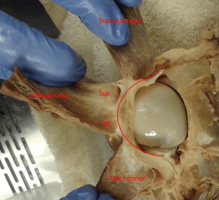
Anatomical Dissection: This clinical photograph provides a posterior view of a dissected left human shoulder, focusing on the rotator cuff complex. The supraspinatus, infraspinatus, and teres minor muscles are reflected laterally to reveal the underlying humeral head and its capsule. A curved red line overlay highlights the rotator cable, a thick fibrous band that spans the avascular zone of the rotator cuff. The infraspinatus muscle is further subdivided with labels 'Sup.' and 'Inf.', representing the superior and inferior portions of the muscle, respectively. The image demonstrates the varying degrees of adherence between the infraspinatus and the rotator cable, illustrating the functional anatomy of the shoulder's capsuloligamentous structures. This material is useful for studying musculoskeletal anatomy, specifically the insertions of the rotator cuff and the biomechanical role of the rotator cable in distributing forces across the shoulder joint.
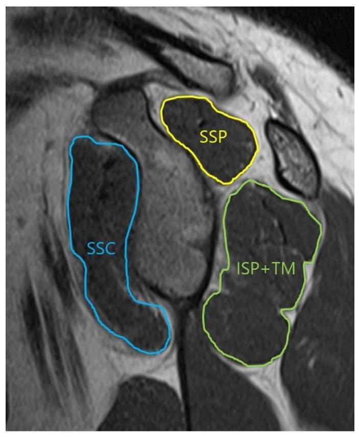
This oblique-sagittal T2 Turbo Spin Echo (TSE) MRI scan demonstrates the musculoskeletal anatomy of the shoulder in a glenoid face view, specifically for assessing the cross-sectional area of the rotator cuff muscles. The image features color-coded annotations outlining the muscular boundaries: the supraspinatus (SSP) is outlined in yellow in the superior position; the subscapularis (SSC) is traced in blue anteriorly; and the infraspinatus combined with the teres minor (ISP+TM) is outlined in green in the posterior-inferior quadrant. The musculature appears as intermediate to dark gray signal intensity, allowing for the evaluation of muscle volume and potential fatty infiltration or atrophy. This imaging view is clinically significant for orthopedic evaluation and preoperative planning in cases of rotator cuff tears or shoulder instability, providing a clear visualization of the muscular support surrounding the glenohumeral joint.
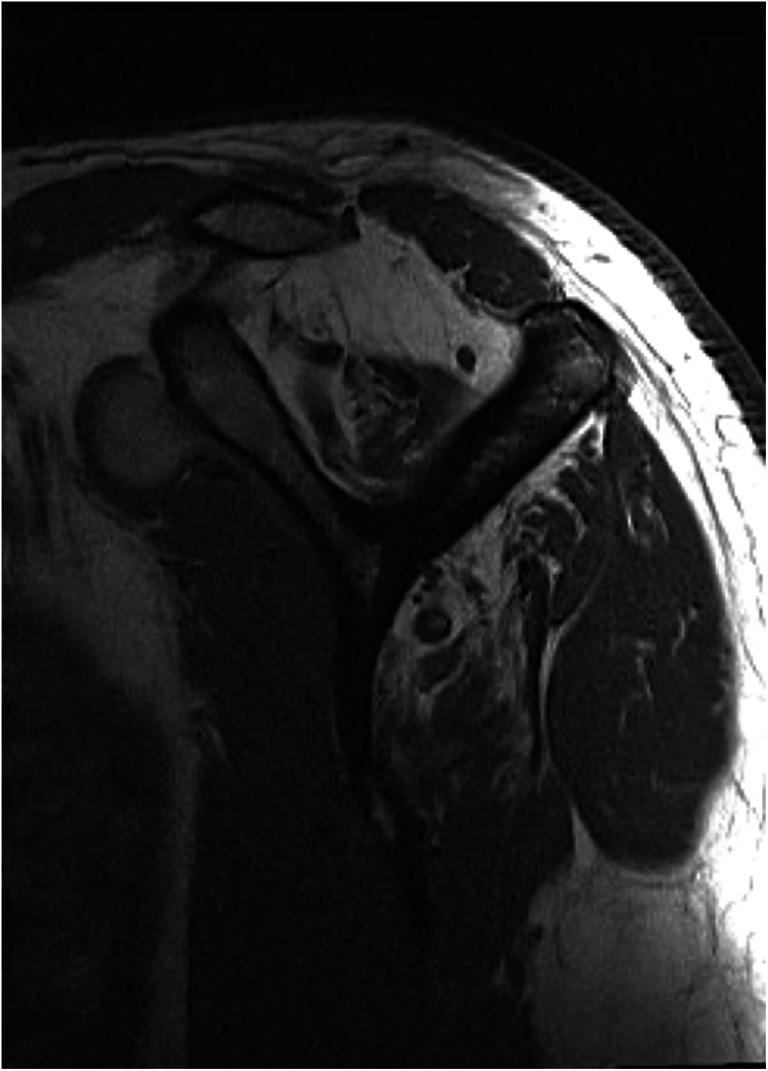
This diagnostic image is a T1-weighted parasagittal MR slice of the shoulder, specifically oriented to evaluate the rotator cuff musculature. The image demonstrates advanced fatty infiltration and muscular atrophy, critical for determining the reparability of chronic rotator cuff tears. The supraspinatus muscle shows a significant loss of muscle bulk (atrophy) and high signal intensity (hyperintensity), indicating replacement of muscle fibers by adipose tissue, consistent with a high Goutallier stage. Similarly, the infraspinatus muscle exhibits marked fatty degeneration. In contrast, the subscapularis and teres minor muscles maintain a normal, low-signal appearance (hypointense) relative to the fat, indicating preserved muscle quality without significant degeneration. This comparison serves as a key clinical indicator in orthopedic radiology for surgical planning and prognosis in patients with tendon pathology.
knee joint anatomy ACL PCL meniscus ligaments
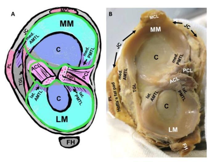
Educational visual showing the gross anatomy and schematic representation of the human tibial plateau and its intraarticular structures. The image is divided into a labeled schematic (A) and a corresponding clinical photograph of a cadaveric specimen (B), demonstrating the spatial relationships of the knee joint. Key anatomical features identified include the medial meniscus (MM) and lateral meniscus (LM) resting on the tibial articular cartilage (C). The cruciate ligaments—anterior (ACL) and posterior (PCL)—are shown centrally. Detailed focus is given to the meniscotibial ligaments, specifically the medial and lateral anterior meniscotibial ligaments (AMTL) and posterior meniscotibial ligaments (PMTL), which provide elastic fixation for the meniscal horns. Additional structures visible include the transverse genicular ligament (TGL) connecting the menisci, the medial collateral ligament (MCL), the joint capsule (JC), and the fibular head (FH). The schematic further illustrates the synovial membrane (green line) and its relation to the joint cavity. This material is designed to teach orthopedic anatomy, emphasizing the complex ligamentous network supporting knee joint stability and the entheses involved in degenerative conditions like osteoarthritis.
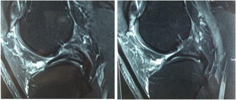
Two sagittal T2-weighted magnetic resonance imaging (MRI) slices of the human knee joint demonstrate a rare anatomical meniscal variant. The diagnostic images show the distal femur, proximal tibia, and the posterior aspect of the knee joint. A prominent feature is the posterior junction and fusion of the medial and lateral meniscal horns. Specifically, fibers from the anterior cruciate ligament (ACL) appear to insert directly into the posterior horn of the lateral meniscus rather than their typical tibial attachment, a condition associated with visible thinning of the primary ACL band. Both the ACL and the posterior cruciate ligament (PCL) are visible as hypointense, dark structures against the hyperintense signal of joint fluid. This imaging is clinically significant for identifying rare congenital variations in meniscal morphology that can predispose patients to mechanical blocking or knee locking symptoms. The visualization highlights the complex relationships between the cruciate ligaments and meniscal attachments within the intra-articular space.
ankle lateral ligaments ATFL CFL anatomy
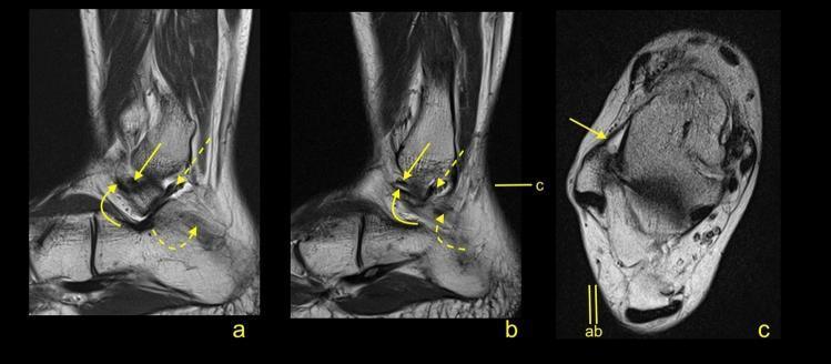
Magnetic Resonance Imaging (MRI) of the ankle joint in a 45-year-old patient, displaying sagittal (a, b) and transverse (c) sections. The images focus on the anatomy of the lateral collateral ligament complex. The sagittal views demonstrate a double-fascicular anterior talofibular ligament (ATFL), characterized by two distinct bundles of approximately equal diameter: the superior fascicle (S-ATFL, indicated by a straight yellow arrow) and the inferior fascicle (I-ATFL, indicated by a curved yellow arrow). The posterior talofibular ligament (PTFL) is visible as a hypointense band marked by a straight dashed arrow, while the calcaneofibular ligament (CFL) is denoted by a curved dashed arrow. In the transverse section (c), the orientation of the ATFL (arrow) relative to the lateral malleolus and talus is shown. These images are used to illustrate normal anatomical variants of the ankle ligaments, specifically the bifid or double-fascicular appearance of the ATFL, which is relevant for accurate diagnostic interpretation of ankle sprains and ligamentous stability.
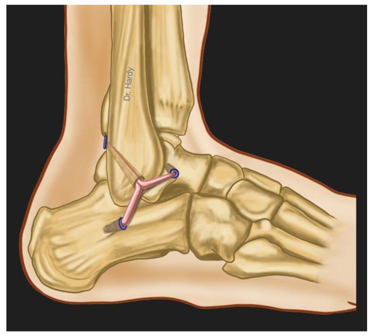
This medical anatomical diagram illustrates an anatomic surgical reconstruction of the lateral ankle ligament complex from a lateral view. The diagram depicts the skeletal structures of the distal fibula, talus, calcaneus, and tarsal bones. The primary focus is the surgical reconstruction of the three main lateral ligaments: the Anterior Talofibular Ligament (ATFL), the Calcaneofibular Ligament (CFL), and the Posterior Talofibular Ligament (PTFL). The reconstruction utilizes a split tendon autograft (such as a gracilis tendon) that is anchored to the distal fibula. The graft bifurcates and extends into three distinct limbs, which are secured into bone tunnels on the talus and calcaneus using blue-colored interference screws or anchors. This illustration demonstrates the surgical technique used to manage chronic lateral ankle instability by replicating the native anatomy of the lateral ligament complex to restore joint stability and biomechanical function.
DAY 1: Musculoskeletal Anatomy
Sports Physiotherapy Lens — Examination Depth
PART 1: THE SHOULDER COMPLEX
1.1 The Four Joints of the Shoulder Complex
| Joint | Type | Key Function |
|---|---|---|
| Glenohumeral (GHJ) | Ball-and-socket (synovial) | Primary mobility — greatest ROM of any joint |
| Scapulothoracic (STJ) | Physiological (not a true synovial joint) | Scapular rotation, positioning the glenoid |
| Acromioclavicular (ACJ) | Plane synovial | Fine-tuning clavicular rotation at end-range abduction |
| Sternoclavicular (SCJ) | Saddle synovial (only true synovial joint of the shoulder girdle connecting to axial skeleton) | Clavicular elevation, depression, protraction |
1.2 Glenohumeral Joint — Architecture
- Glenoid labrum — a fibrocartilaginous rim that deepens the socket by ~50%, increasing contact area. The labrum contributes 10mm of additional depth. Bankart lesion = anteroinferior labral tear (anterior instability mechanism).
- Glenohumeral ligaments (GHL) — thickenings of the anterior capsule:
- Superior GHL: resists inferior translation in adduction
- Middle GHL: resists anterior translation at 45–60° abduction
- Inferior GHL (IGHL) — the most important: primary restraint to anterior translation at 90° abduction + ER. This is the ligament stressed in the late cocking phase of throwing. The anterior band of IGHL is the primary restraint in the position of apprehension.
- Coracohumeral ligament: resists inferior subluxation and ER in adduction
1.3 The Rotator Cuff — Anatomy That Drives the Exam
| Muscle | Origin | Insertion | Innervation | Primary Action | Key Exam Point |
|---|---|---|---|---|---|
| Supraspinatus | Supraspinous fossa | Greater tubercle (superior facet) | Suprascapular n. (C5,6) | Initiates abduction (0–15°), assists deltoid throughout | FIRST muscle active in abduction; most commonly torn |
| Infraspinatus | Infraspinous fossa | Greater tubercle (middle facet) | Suprascapular n. (C5,6) | External rotation (primary); posterior GHJ stability | Atrophies in suprascapular nerve entrapment |
| Teres minor | Lateral border scapula | Greater tubercle (inferior facet) | Axillary n. (C5,6) | External rotation, inferior translation | Tested in IR deficit (GIRD context) |
| Subscapularis | Subscapular fossa | Lesser tubercle | Upper + lower subscapular n. (C5,6,7) | Internal rotation (primary); anterior stability | Lift-off test / belly press test |
- Deltoid = superior translatory force (destabilising)
- Infraspinatus + Teres minor + Subscapularis = inferior compressive force (stabilising)
- This is the transverse force couple at the GHJ
1.4 Scapulothoracic Rhythm — The 2:1 Rule
- 2° occurs at the GHJ
- 1° occurs at the STJ (scapular upward rotation)
- Upward rotators of scapula: Serratus anterior (SA) + Upper + Lower trapezius
- SA = single most important muscle for scapular upward rotation and protraction; innervated by long thoracic nerve (C5,6,7)
- Winging of scapula = serratus anterior palsy (long thoracic nerve injury) — medial border lifts off thorax on pushing test
1.5 GIRD — Glenohumeral Internal Rotation Deficit
- Posterior capsule contracts (posterior capsular tightness/thickening)
- Anterior capsule stretches (increased laxity)
- Net effect: entire GHJ arc shifts posteriorly — ER increases, IR decreases
- Internal impingement (supraspinatus + infraspinatus compressed against posterosuperior glenoid rim during late cocking)
- Increased SLAP tear risk (posterosuperior labrum)
- Increased partial-thickness articular-side rotator cuff tear risk
- Measured in supine, shoulder at 90° abduction, stabilise scapula (prevent scapular anterior tipping), measure IR passively
- GIRD = dominant IR minus non-dominant IR (if >18–20° = clinically significant)
- Total arc of motion (TROM): ER + IR = should be equal in both shoulders (normally ~170–180°). If TROM is reduced on throwing side, posterior capsule is tight. If TROM is equal but arc has shifted (more ER, less IR), it may reflect bony adaptation (humeral retroversion) rather than capsular tightness.
PART 2: THE KNEE
2.1 Bony Architecture
- Medial tibiofemoral
- Lateral tibiofemoral
- Patellofemoral
2.2 The Cruciate Ligaments
- Origin: Posterior medial surface of lateral femoral condyle (in the intercondylar notch)
- Insertion: Anterior intercondylar area of tibial plateau (anterior to tibial spine)
- Direction: Runs anteriorly, medially, and distally from femur to tibia
- Two functional bundles:
- Anteromedial (AM) bundle — taut in flexion, primary restraint to anterior tibial translation
- Posterolateral (PL) bundle — taut in extension, provides rotational stability
- Primary function: Resist anterior tibial translation on femur; resist internal tibial rotation
- Blood supply: Middle genicular artery (why it heals poorly — intrasynovial location with limited vascular supply)
- Innervation: Branches of tibial nerve (mechanoreceptors → proprioception; this is why proprioceptive deficits persist after ACL injury)
- Origin: Lateral surface of medial femoral condyle
- Insertion: Posterior intercondylar area (posterior tibial plateau)
- Stronger than ACL (twice the tensile strength)
- Primary function: Resist posterior tibial translation; "cornerstone" of knee stability
- Mechanism of injury: Dashboard injury (posterior force on proximal tibia with knee flexed = PCL tear)
2.3 The Menisci
| Feature | Medial Meniscus | Lateral Meniscus |
|---|---|---|
| Shape | C-shaped (open semicircle) | O-shaped (nearly circular) |
| Size | Covers ~60% of medial tibial plateau | Covers ~80% of lateral tibial plateau |
| Mobility | Less mobile (more firmly attached to capsule + MCL) | More mobile (only attached at horns) |
| Injury frequency | More commonly injured | Less commonly injured |
| Peripheral vascularity | Red-red zone (outer 1/3) — heals; Red-white zone (middle 1/3) — variable; White-white zone (inner 2/3) — avascular, does not heal | Same zonal pattern |
- Load distribution — without menisci, 70% of medial compartment contact stress concentrated on articular cartilage (menisci distribute it across 50% of total area)
- Shock absorption — reduce peak forces by ~20%
- Joint stability — secondary restraint to anterior tibial translation (explains why isolated ACL + meniscus tears cause more instability than ACL alone)
- Lubrication and nutrition of articular cartilage
- Proprioception (mechanoreceptors in meniscal tissue)
2.4 Collateral Ligaments
- Superficial layer: tibial collateral ligament (long, from medial femoral epicondyle to medial tibia)
- Deep layer: middle capsular ligament (attached to medial meniscus — explains why MCL injury can tear medial meniscus)
- Resists valgus stress and external tibial rotation
- Extrasynovial → good blood supply → heals well conservatively
- Fibular collateral ligament: from lateral femoral epicondyle to fibular head
- Cord-like, not attached to lateral meniscus
- Resists varus stress
- Part of the posterolateral corner (PLC) complex with popliteus, popliteofibular ligament
2.5 The Extensor Mechanism and Patellofemoral Joint
- Increases lever arm of quadriceps by ~50% (moves tendon force away from knee axis)
- Reduces friction by distributing compressive forces across trochlear groove
- Protects anterior knee
- Walking: ~0.5x body weight
- Stair descent: ~3.3x body weight
- Deep squat: ~7–8x body weight
- This explains why patellofemoral pain is aggravated by stairs, squatting, and prolonged sitting (patella tracks against trochlea with knee flexed)
- Vastus medialis oblique (VMO) fibers insert at 50–55° to the long axis of quadriceps
- VMO is the only muscle providing a medial component of pull on the patella (countering the lateral pull of vastus lateralis + ITB + retinaculum)
- VMO atrophies early and selectively in patellofemoral pain syndrome (PFPS) and knee OA
- Q-angle: Angle between line from ASIS to patella centre and line from patella centre to tibial tuberosity
- Normal: males ~10–15°, females ~15–20° (wider pelvis → higher Q-angle → greater lateral patellar pull)
- Q-angle >20° = increased PFPS risk (direct sample question answer justification)
PART 3: THE ANKLE AND FOOT
3.1 The Ankle Joint (Talocrural Joint)
- Medial malleolus (tibia) + Lateral malleolus (fibula) + Tibial plafond (inferior articular surface of tibia) forming the "fork/mortise"
- Talus = the "tenon" that sits in the mortise
- In dorsiflexion: wider part engaged → mortise spreads → joint is MOST STABLE (locked position)
- In plantarflexion: narrower part engaged → mortise less snug → joint is LEAST STABLE
- This is why lateral ankle sprains occur in plantarflexion + inversion — the joint is in its most unstable position
3.2 Lateral Ankle Ligaments — The Most Injured Ligaments in Sport
| Ligament | From | To | Injury Order | Function |
|---|---|---|---|---|
| ATFL (anterior talofibular) | Anterior fibula | Lateral talar neck | First and most commonly torn (~85% of ankle sprains) | Resists plantarflexion + inversion; primary restraint when foot is plantarflexed |
| CFL (calcaneofibular) | Fibular tip | Lateral calcaneus | Second to tear (with more severe sprains) | Resists inversion in neutral/dorsiflexion; crosses both talocrural and subtalar joints |
| PTFL (posterior talofibular) | Posterior fibula | Posterior talus | Rarely torn — only in complete dislocation | Resists posterior displacement of talus |

3.3 Sever's Disease — Calcaneal Apophysitis
- Achilles tendon inserts into the posterior calcaneal tuberosity
- With running and jumping, the Achilles exerts repetitive tensile forces through the apophysis
- The unfused apophysis cannot handle these repetitive traction loads → microtrauma → inflammation → Sever's disease
- Plantar fasciitis: pain at plantar medial calcaneal tuberosity (origin of plantar fascia)
- Achilles tendinopathy: pain 2–6cm above calcaneal insertion (mid-tendon) or at insertion (insertional)
- Sever's: pain at posterior calcaneal apophysis (growth plate region)
3.4 Plantar Fascia and Achilles Tendon
- Origin: Medial calcaneal tuberosity
- Insertion: Base of proximal phalanges (via plantar plates)
- Function: Windlass mechanism — during toe extension (push-off), plantar fascia tightens, raising the arch, converting foot into a rigid lever for propulsion
- Clinical: Plantar fasciitis = degeneration/inflammation at calcaneal origin; most painful with first steps in morning (fascia stiffens overnight, then is suddenly loaded)
- Common tendon of gastrocnemius + soleus (triceps surae)
- Inserts into middle posterior calcaneus
- Critical zone: 2–6cm proximal to insertion = watershed zone (relative avascularity) → most common site of rupture and non-insertional tendinopathy
- Gastrocnemius crosses the knee (knee flexion weakens it); soleus does not (pure ankle plantarflexor regardless of knee position)
- Thompson test (calf squeeze test): Squeeze calf → normally produces plantarflexion. Absence of plantarflexion = complete Achilles rupture.
PART 4: THE HIP AND THIGH
4.1 Hip Joint
- Acetabulum covers ~170° of femoral head (vs. 30% at GHJ)
- Acetabular labrum deepens the socket (like shoulder labrum)
- Femoral head is supplied by:
- Medial circumflex femoral artery (dominant supply to femoral head) — runs posterior along femoral neck
- Lateral circumflex femoral artery
- Ligamentum teres artery (minor, significant only in children)
- Normal neck-shaft angle (NSA): ~126–128° in adults
- Coxa vara: NSA <120° → limb shortening, Trendelenburg gait
- Coxa valga: NSA >140° → increased bending stress on femoral neck
4.2 The Hamstrings — Your Most Tested Thigh Anatomy
| Muscle | Origin | Insertion | Innervation | Action |
|---|---|---|---|---|
| Biceps femoris (long head) | Ischial tuberosity (common tendon with semitendinosus) | Fibular head | Tibial division of sciatic (L5-S2) | Knee flexion, hip extension, external tibial rotation |
| Biceps femoris (short head) | Lateral lip of linea aspera | Fibular head | Common peroneal division of sciatic (L5-S1) | Knee flexion, external tibial rotation (NO hip extension — doesn't cross hip) |
| Semitendinosus | Ischial tuberosity | Pes anserinus (medial tibia — with gracilis and sartorius) | Tibial division (L5-S2) | Knee flexion, hip extension, internal tibial rotation |
| Semimembranosus | Ischial tuberosity | Posterior medial tibial condyle | Tibial division (L5-S2) | Knee flexion, hip extension, internal tibial rotation |
- Biarticular muscle — crosses both hip and knee, subject to large eccentric loads during late swing phase of sprinting (hip flexing + knee extending simultaneously = maximum stretch under load)
- Transition zone vulnerability — the musculotendinous junction (MTJ) of the long head is the most common site of grade 2/3 strain
- Two-nerve supply distinction: Long head (tibial division) vs. short head (common peroneal division) — this is an exam-favourite neuroanatomy question
- During sprinting: At late swing phase, hamstrings act eccentrically to decelerate knee extension while simultaneously initiating hip extension for ground contact. This is the peak load position.
4.3 Hip Stabilisers and Trendelenburg Mechanism
PART 5: THE SPINE
5.1 Vertebral Column — Structure and Regional Characteristics
- Cervical: lordosis (concave posteriorly) — 7 vertebrae
- Thoracic: kyphosis (concave anteriorly) — 12 vertebrae
- Lumbar: lordosis — 5 vertebrae
- Sacral: kyphosis (fixed) — 5 fused vertebrae
5.2 Intervertebral Disc — Structure and Pathomechanics
- Nucleus pulposus: Central gelatinous core — 70–90% water in youth; highly hydrophilic (proteoglycans bind water). Behaves as a fluid under compression (Pascal's law: transmits pressure equally in all directions). Derived from the notochord.
- Annulus fibrosus: Concentric lamellae of type I collagen fibres; adjacent layers alternate direction (~30° to disc plane, opposing directions). Posterior fibres are thinner and more susceptible to herniation.
- Endplates: Hyaline cartilage; nutrients diffuse from vertebral body through endplate into disc (avascular disc in adults depends on diffusion)
- The nucleus migrates posterolaterally (path of least resistance — posterior annulus thinner + posterior longitudinal ligament narrow)
- Posterolateral herniation → compresses nerve root in intervertebral foramen
- L4-L5 disc → L5 nerve root (walks in intervertebral foramen)
- L5-S1 disc → S1 nerve root (most common clinical level)
- L3: medial thigh
- L4: medial leg + medial foot (big toe dorsum)
- L5: Lateral leg + dorsum of foot + great toe (tests EHL strength)
- S1: Lateral/plantar foot + little toe (tests ankle plantarflexion, Achilles reflex)
- C5: lateral upper arm
- C6: lateral forearm + thumb (biceps reflex)
- C7: middle finger (triceps reflex)
- C8: medial forearm + little finger
5.3 Lumbar Spine — Sports-Relevant Anatomy
- Lumbar facets are oriented in the sagittal plane (~45° to transverse plane) → allow flexion-extension and lateral flexion, but restrict rotation
- Thoracic facets are near-frontal plane → allow rotation, restrict flexion
- This is why lumbar rotation is limited (~5° per level) and thoracic rotation is the primary rotational segment
- Transversus abdominis (TrA): Deep abdominal muscle, activates ~30ms BEFORE limb movement in healthy subjects (anticipatory/feedforward activation). Atrophies in chronic LBP.
- Multifidus: Deep erector spinae; segmental stabiliser. Atrophies ipsilaterally and selectively in LBP and remains atrophied even after pain resolves (clinical implication: must be specifically retrained).
- Superficial erectors (iliocostalis, longissimus): Global movers, generate large forces; not segmental stabilisers.
PART 6: NEUROANATOMY OF THE UPPER LIMB — Key Peripheral Nerves
| Nerve | Root | Vulnerable Site | Injury Result | Clinical Test |
|---|---|---|---|---|
| Axillary nerve | C5,6 | Posterior shoulder (GHJ dislocation, surgical neck fracture) | Deltoid paralysis, lateral shoulder sensory loss | Deltoid testing, "regimental badge" area |
| Musculocutaneous | C5,6,7 | Coracobrachialis muscle | Biceps + brachialis weakness, lateral forearm sensory loss | Biceps curl weakness |
| Radial nerve | C5-T1 | Spiral groove of humerus (mid-shaft humeral fracture) | Wrist drop (finger + wrist extension lost) | Wrist/finger extension |
| Median nerve | C6-T1 | Carpal tunnel (most common compression neuropathy) | "Ape hand" (loss of thenar eminence), loss of thumb opposition, lateral 3.5 fingers sensory loss | Phalen's, Tinel's at wrist |
| Ulnar nerve | C8-T1 | Cubital tunnel (medial epicondyle) | Claw hand (4th, 5th fingers), hypothenar wasting, loss of all intrinsics | Froment's sign, Wartenberg's |
| Long thoracic nerve | C5,6,7 | Along lateral chest wall (serratus anterior) | Medial scapular winging | Wall push-up test |
| Suprascapular nerve | C5,6 | Suprascapular notch or spinoglenoid notch | Supraspinatus + infraspinatus atrophy/weakness | ER weakness, infraspinatus hollow |
SAMPLE-STYLE MCQs — Day 1 Self-Test
ANSWERS WITH MECHANISMS
HIGH-YIELD SUMMARY — Review the Night Before
- Rotator cuff order: SITS | Supraspinatus initiates abduction (0–15°)
- Most important GHJ stabiliser ligament at 90° ABD+ER = IGHL anterior band
- GIRD = posterior capsule tight = >18–20° IR loss = throws cause it = sleeper stretch treats it
- Subacromial space = coracoacromial arch above + humeral head below; Bigliani Type III = hooked = impingement
- Scapulohumeral rhythm = 2:1 (GHJ:STJ)
- ACL origin = lateral femoral condyle POSTERIOR surface; insertion = anterior tibial plateau
- Lachman test = most sensitive for ACL (90% sensitivity at 20–30° flexion)
- Medial meniscus more commonly injured; lateral meniscus more mobile
- VMO atrophies selectively in PFPS; Q-angle >20° = lateral patellar pull
- PFJRF at stair descent = ~3.3x BW; deep squat = ~7x BW
- ATFL torn first (plantarflexion + inversion); talus wider anteriorly = PF is least stable position
- Sequence of lateral ligament injury: ATFL → CFL → PTFL
- Biceps femoris long head = most commonly injured; eccentrically loaded at late swing phase
- Short head = ONLY hamstring not crossing hip; innervated by COMMON PERONEAL (not tibial)
- Semitendinosus inserts at pes anserinus (with sartorius and gracilis)
- Disc: Nucleus pulposus (notochordal origin) + annulus fibrosus (type I collagen)
- Herniation most common posterolateral; L5-S1 → S1 root (Achilles reflex, plantarflexion)
- TrA + multifidus = deep stabilisers; multifidus atrophies selectively in LBP
- Spondylolysis = pars stress fracture = young athlete + hyperextension sport
- Shoulder complex — 4 joints, rotator cuff force couples, IGHL, GIRD mechanism and measurement, scapulohumeral rhythm
- Knee — ACL/PCL (origin/insertion/bundles), meniscal anatomy and function, collateral ligaments, extensor mechanism, Q-angle, PFJRF
- Ankle and foot — talocrural joint, lateral ligament sequence (ATFL → CFL → PTFL), Sever's disease mechanism, plantar fascia windlass mechanism, Achilles watershed zone
- Hip and thigh — hamstring anatomy (the two-nerve rule for biceps femoris), pes anserinus, Trendelenburg mechanism
- Spine — disc structure, herniation pathomechanics, dermatomes, pars interarticularis, deep stabiliser muscles