
CT times
What do you mean by 'CT times'?
- CT scan timing/protocols - things like contrast phase timing (arterial, venous, delayed), scan duration, or when contrast should be administered relative to injection
- Central Time (CT) - the current time in the US Central time zone
- Something else entirely (please specify)
1
CT scan contrast phase timing protocol arterial portal venous delayed seconds
CT Contrast Phase Timing
Standard phases (from contrast injection start)
| Phase | Typical timing | What it shows |
|---|---|---|
| Non-contrast (baseline) | 0 s | Baseline density, calcifications, hemorrhage, stones |
| Early arterial phase | ~15-20 s (or 10-15 s post bolus-track trigger) | Pure arterial anatomy, CT angiography, active bleeding/extravasation |
| Late arterial phase (a.k.a. "arterial phase" or "early portal venous phase") | ~30-40 s (25-45 s window); with bolus tracking, 15-20 s after trigger | Hypervascular tumors (HCC, neuroendocrine tumors, pancreatic adenocarcinoma conspicuity), pancreatic parenchymal phase |
| Portal venous phase | ~60-80 s (commonly quoted 70-80 s) | General abdominal survey - best combined solid organ, bowel wall, and vascular enhancement; detects hypovascular liver metastases; most "routine" abdominal CTs are done here |
| Nephrographic/nephrogenic phase | ~90-120 s | Renal parenchymal enhancement, renal mass characterization |
| Delayed/equilibrium phase | ~3-5 min (up to 10 min) | Washout characterization of HCC, hemangiomas, cholangiocarcinoma, delayed excretory renal phase, active contrast extravasation pooling |
| Excretory (urographic) phase | ~5-15 min | Contrast in collecting system/ureters for CT urography |
"the minimum requirement for liver imaging is typically a relatively late arterial phase (e.g. centred 18 s post contrast medium arrival in the abdominal aorta) and a portal venous phase" - Grainger & Allison's Diagnostic Radiology, p. 621 (approx.)
Region-specific notes
- Liver/HCC protocol: non-contrast -> late arterial (~35 s) -> portal venous (~75-80 s) -> sometimes delayed (~5 min), since HCC's classic signature is arterial hyperenhancement with washout on portal/delayed phases.
- Pancreas protocol: late arterial/pancreatic phase (~35-40 s) for tumor detection, plus portal venous phase (~65-70 s) for staging/vascular involvement.
- Renal mass/stone protocol: non-contrast is essential (stones, baseline density), followed by nephrographic (~90-120 s) and sometimes delayed excretory phase for collecting-system evaluation.
- CT angiography (PE, aortic dissection, trauma): bolus-tracked arterial timing (trigger threshold in the target vessel, typically 100-150 HU), scan starts 4-6 s after trigger - much earlier than routine arterial phase, since the goal is peak vessel opacification, not parenchymal enhancement.
- 4D CT (parathyroid): precontrast -> arterial phase -> delay phase (60-80 s post injection), exploiting parathyroid tissue's rapid arterial uptake and rapid washout versus thyroid tissue - Sabiston Textbook of Surgery, ch. 74.
Practical determinants of timing
- Bolus tracking (region-of-interest placed in aorta/vessel, scan triggers automatically at a set HU threshold) is now standard for arterial-phase precision, since the arterial window is brief and mistiming can render a study non-diagnostic for hypervascular lesion detection.
- Injection rate (typically 3-5 mL/s) and contrast volume/concentration shift these windows - faster injection reaches peak arterial enhancement sooner.
- Scanner speed (multi-slice/detector count) affects when you start the acquisition relative to the target phase, since a fast scanner covering the whole liver in a few seconds can start slightly later than a slower scanner needing more acquisition time to still center the acquisition on the target phase.
CT contrast calculation
CT contrast volume dose calculation formula mL/kg iodine delivery rate injection rate
CT Contrast Dose/Volume Calculation
1. Weight-based volume (most common bedside method)
| Patient weight | Contrast volume |
|---|---|
| <75 kg | 100 mL |
| 75-90 kg | 120 mL |
| >90 kg | 150 mL |
2. Iodine-dose-based calculation (more physiologic, adjusts for contrast concentration)
Total iodine dose (g) = target load (gI/kg) x weight (kg)
Volume (mL) = Total iodine dose (mg) / concentration (mgI/mL)
- Total iodine needed = 0.45 x 70 = 31.5 gI = 31,500 mg
- Volume = 31,500 / 370 = ~85 mL
3. Flow rate and injection duration
Volume (mL) = Flow rate (mL/s) x Duration (s)
4. Iodine Delivery Rate (IDR) - governs arterial enhancement peak
IDR (gI/s) = concentration (mgI/mL) x flow rate (mL/s) / 1000
5. Adjustments and safety caps
- Renal function: Contrast volume/iodine dose is capped or reduced in patients with reduced eGFR to lower contrast-induced nephropathy (CIN/PC-AKI) risk; many institutions cap total iodinated load or require isotonic saline pre-hydration below an eGFR threshold (commonly <30-45 mL/min/1.73m²).
- Cardiac output/heart rate: In CT angiography protocols (e.g. cardiac CT), injected volume is adjusted upward for higher heart rates (contrast transits faster) - e.g. +10-30 mL correction for heart rates above 65 bpm in some validated formulas (iCalc-type models).
- Body surface area (BSA) is sometimes used instead of weight alone for more individualized dosing (e.g., ~45 mL/m² as a baseline, per Yanaga's model), particularly for cardiac/CTA protocols.
- Saline flush (30-40 mL at the same flow rate) is added after the contrast bolus to push the trailing contrast column out of peripheral veins into central circulation, improving enhancement efficiency and reducing wasted contrast.
Worked example
- Volume = 100 mL (weight <75 kg)
- Flow rate = 3-4 mL/s -> injection time ~25-33 s
- Total iodine dose = 100 mL x 350 mg/mL = 35 g iodine
- IDR at 3.5 mL/s = 350 x 3.5/1000 = 1.23 gI/s (adequate for portal venous phase; would push flow rate to 5 mL/s for arterial-phase/HCC protocol)
MRI mrcp planing
MRCP sequence planning protocol slice positioning coronal oblique technique
MRCP Planning (Sequence Positioning & Protocol)
Standard scan sequence order
- Three-plane localizer to establish reference anatomy.
- Axial T2 HASTE/TRUFISP (fat-sat), respiratory-triggered or breath-hold through the liver and pancreas - this is the key localizer image used to identify the course of the common bile duct (CBD) for planning the oblique MRCP slabs.
- Axial T1 gradient echo, in/out-of-phase with fat suppression - for parenchymal (liver/pancreas) lesion characterization.
- Coronal T2 HASTE/TRUFISP thin slices covering the whole liver (anterior abdominal wall to paraspinal muscles).
- Coronal oblique thick-slab MRCP (single-slice, "projection" MRCP) - the signature MRCP image.
- Coronal oblique thin-slice 3D MRCP (SPACE/FRFSE-based, respiratory-gated) for a true source-image dataset that can be reconstructed/MIP'd.
Planning the coronal oblique thick-slab MRCP (the key step)
- Plan on the axial T2 HASTE/TRUFISP image that clearly shows the CBD in cross-section.
- Position the thick slab (typically 40 mm) across the CBD, then rotate:
- RAO (right anterior oblique), rotate ~20-30° counterclockwise to include both the CBD and the pancreatic duct in the same slab (this is the "classic" MRCP projection).
- LAO (left anterior oblique), rotate ~20-30° clockwise to include the CBD and gallbladder together.
- Verify the slab position in the other two planes (sagittal/coronal) before acquiring, adjusting the sagittal angle so it runs horizontally through the duct.
- Use phase oversampling (~50%) on the coronal obliques to prevent wrap-around artifact from the arms/lateral abdominal wall.
- Apply fat saturation if the patient's breathing pattern is irregular (switch to a multi-NEX free-breathing fat-sat technique instead of respiratory triggering).
Typical parameters (single-slice thick-slab T2 HASTE MRCP)
| Parameter | Typical value |
|---|---|
| TR | 3000-4000 ms (some protocols use as low as 1000-1500 for HASTE variants) |
| TE | ~100-110 ms (long TE to suppress background, keep only fluid bright) |
| Flip angle | ~150° |
| Slice thickness | 40 mm single thick slab (projection MRCP) or 3-5 mm for thin-slice/3D |
| Matrix | 320 x 320 |
| FOV | 400-450 mm |
| Phase direction | A>P (axial) or R>L (coronal oblique) |
| Oversampling | 50% |
| NEX | 1 |
3D MRCP (thin-slice, respiratory-navigated)
- Planned as a coronal oblique block over the biliary tree, typically 6 mm slice thickness with 1 mm gap, 32-38 slices, covering from the hepatic dome down through the kidneys/pancreatic head-body-tail.
- Uses respiratory navigator/triggering (not breath-hold) since acquisition time is longer, giving higher resolution source images that can be post-processed into MIP reconstructions from any angle - this is the dataset surgeons/gastroenterologists actually review for stone burden, stricture length, and ductal anatomy variants.
- Patient positioned supine, feet-first, abdomen at isocenter; arms up if possible to reduce fold-over artifact on coronal sequences.
Clinical relevance of MRCP planning quality
With image
MRCP magnetic resonance cholangiopancreatography image showing bile duct pancreatic duct
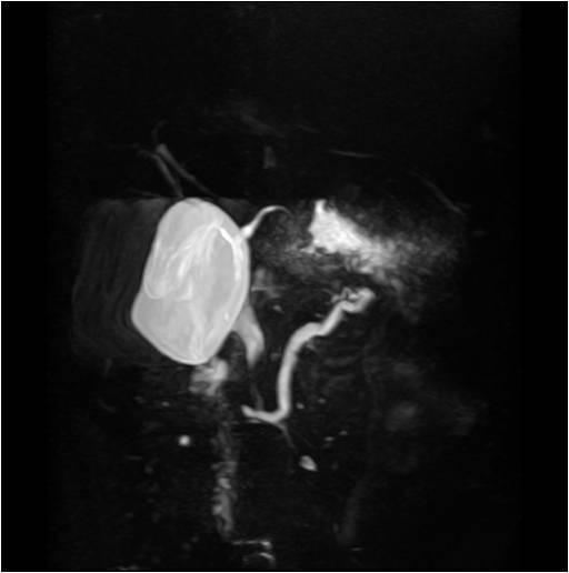
This diagnostic image is a Magnetic Resonance Cholangiopancreatography (MRCP) showing the biliary and pancreatic ductal systems. The primary finding is pancreas divisum, a congenital anatomical variant where the dorsal and ventral pancreatic ducts fail to fuse. The image demonstrates a prominent, slightly dilated dorsal pancreatic duct that crosses over the common bile duct to drain into the minor papilla. A focal narrowing or stenosis is visible at the level of the minor papilla. In contrast, the ventral pancreatic duct appears smaller and normal in morphology, draining separately into the major papilla without any communication with the dorsal duct. The gallbladder and common bile duct are also visualized, with the latter showing mild dilatation. This MRCP finding is clinically significant for diagnosing pancreas divisum, which can be associated with recurrent pancreatitis or obstructive symptoms if drainage through the minor papilla is impaired.
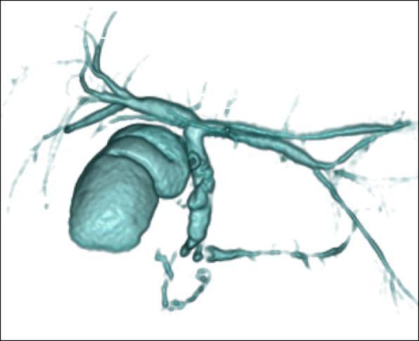
This diagnostic image is a 3D reconstruction from Magnetic Resonance Cholangiopancreatography (MRCP) showing the biliary and pancreatic duct systems. The gallbladder is visualized as a distended, lobulated sac-like structure connected to the biliary tree. The intrahepatic bile ducts appear as a branching network draining into the common bile duct. A significant anatomical variant is demonstrated where the main pancreatic duct forms an annular configuration, encircling the projected location of the second portion of the duodenum. A distinct filling defect is visible within the pancreatic duct at the level of the pancreatic head, likely representing a pancreatic calculus. Distal to this obstruction, the pancreatic duct shows mild compensatory dilatation. The image is clinically relevant for diagnosing congenital anomalies such as annular pancreas and associated complications like obstructive pancreatolithiasis or pancreaticobiliary maljunction.
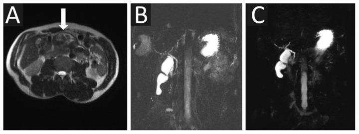
This composite of magnetic resonance imaging (MRI) scans highlights diagnostic findings in a 35-year-old male with a pancreatic pseudocyst. Image A is an axial T2-weighted abdominal scan showing a pancreatic pseudocyst (indicated by a white arrow) characterized by an atypical low or mixed-low signal intensity, located in the peripancreatic region. Images B and C present Magnetic Resonance Cholangiopancreatography (MRCP) views in 2D and 3D formats, respectively. Both MRCP modalities demonstrate high-signal (bright) intensity within the biliary tree, including the gallbladder, cystic duct, and common bile duct. The 3D MRCP in panel C offers superior spatial resolution and anatomical detail compared to the 2D reconstruction in panel B. Notably, neither MRCP sequence successfully visualizes the cystic lesion or its communication with the main pancreatic duct, illustrating potential limitations of standard MRCP in detecting certain pseudocysts that present with low T2 signal intensity. These images are essential for understanding the comparative utility of different MRI sequences in hepatobiliary and pancreatic pathology.
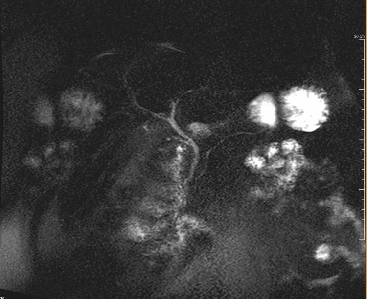
This diagnostic image is a Magnetic Resonance Cholangiopancreatography (MRCP) scan, a specialized MRI modality used to visualize the biliary and pancreatic ducts. The image provides a clear view of the extrahepatic biliary tree, showing a common bile duct (CBD) of normal caliber and a visible pancreatic duct. Notably, there is a remnant cystic duct present, which is consistent with the patient's history of a prior cholecystectomy. The biliary tree appears smooth without evidence of filling defects, such as choledocholithiasis (bile duct stones), or significant ductal dilation (strictures). The high signal intensity typical of fluid-filled structures on T2-weighted MRCP sequences allows for the assessment of ductal patency and morphology. This visual is representative of a normal postoperative biliary anatomy in a clinical workup for acute pancreatitis, where biliary obstruction has been ruled out as the primary etiology.
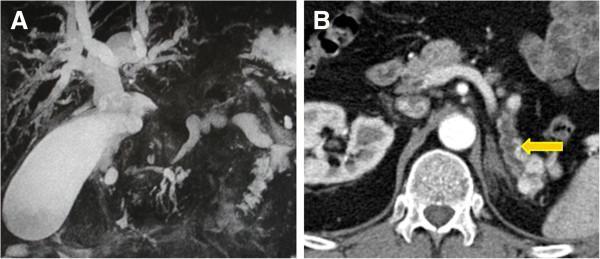
This composite diagnostic image illustrates secondary complications of pancreatic pathology, specifically ductal obstruction. Panel A is a Magnetic Resonance Cholangiopancreatography (MRCP) showing a significant dilatation of the intrahepatic and extrahepatic biliary tree. There is a marked expansion of the common bile duct and gallbladder, secondary to a distal obstruction. The branching bile ducts appear thickened and tortuous, indicating high-pressure upstream effects. Panel B is an axial contrast-enhanced CT scan of the abdomen showing a dilated main pancreatic duct, indicated by a yellow arrow. The pancreatic duct exhibits distal dilatation with a beaded or irregular morphology, a finding commonly associated with proximal mass lesions or chronic obstructive changes. Together, these images demonstrate 'double duct sign' characteristics, where both biliary and pancreatic drainage systems are compromised, frequently seen in periampullary or pancreatic head tumors such as metastases or primary carcinoma.
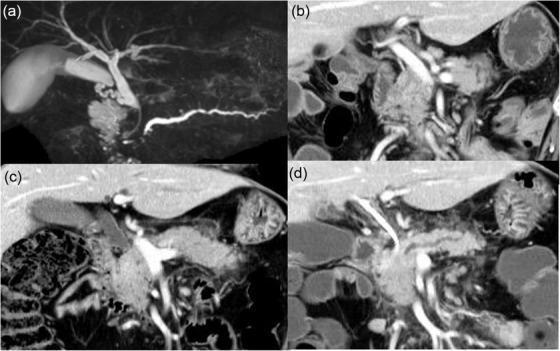
This composite figure displays diagnostic imaging of the hepatobiliary and pancreatic systems. Image (a) is a Magnetic Resonance Cholangiopancreatography (MRCP) demonstrating significant stenosis of the distal common bile duct and the distal main pancreatic duct, resulting in proximal ductal dilation (double-duct sign). A linear radiopaque plastic stent is visible within the common bile duct. Images (b), (c), and (d) are coronal CT scans showing the temporal progression of pancreatic pathology. Image (b) shows the baseline appearance. Image (c), acquired 11 months later, reveals diffuse swelling (hypertrophy) of the entire pancreatic parenchyma. Image (d) illustrates subsequent disease evolution, characterized by swelling localized to the pancreatic head, while the body and tail exhibit atrophic changes. Significant peripancreatic soft tissue infiltration is also noted in (d). This series is clinically relevant for evaluating secondary pancreatic involvement and biliary obstruction, typically seen in metastatic disease or progressive pancreatic conditions.
MRCP coronal oblique slice planning positioning biliary tree
I want imagine planing for technologist
MRI scanner console screen slice positioning localizer planning box technologist
MRCP planning technologist localizer coronal oblique slab positioning screenshot

How to read this image as a technologist
- Some angles cleanly show the CBD and pancreatic duct together (closer to the RAO 20-30° rotation described earlier)
- Other angles bring in more of the gallbladder or lose part of the pancreatic duct out of the slab
- The "best" angle is the one where the CBD, pancreatic duct, and relevant gallbladder anatomy all stay within the slab without the duct exiting the slice plane obliquely (which causes signal dropout/discontinuity)
- Get the axial localizer through the CBD.
- Draw the slab across the duct.
- Rotate (not just translate) the slab 20-30° until the whole ductal course lines up within the slab thickness, checking with a quick single-slice thick-slab acquisition before committing to the longer 3D sequence.
- Cross-check position on the sagittal and coronal planes before finalizing.
Abdomen Cor planing for technician
MRI abdomen coronal localizer slice planning positioning liver kidneys
MRI abdomen coronal sequence planning technologist localizer positioning screenshot liver kidneys
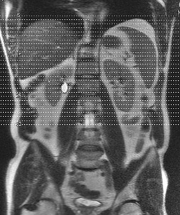
How abdomen coronal planning works for the technologist
- Supine, head-first, spine coil under the patient + body/phased-array coil over the abdomen (xiphoid to anterior superior iliac spine).
- Straps tightened over the coil to reduce respiratory motion artifact.
- Laser landmark centered at the lower intercostal margin (roughly xiphoid level) so the coronal FOV is centered correctly on first shot.
- Right-click/drag the slice block onto the axial localizer image.
- Slice acquisition direction: anterior to posterior.
- Alignment: straight, no angulation needed for a standard coronal abdomen series (unlike MRCP obliques).
- Anatomic coverage: from the anterior liver margin through the posterior kidneys - this ensures the whole liver, spleen, pancreas, and both kidneys are captured within the slab.
- Typical parameters: 4-6 mm slice thickness, 1 mm gap, matrix ~256-320, FOV 350-400 mm, phase direction usually A>P or R>L depending on sequence to push ghosting artifact from lungs/heart or bowel out of the anatomy of interest.
- For liver-focused coronal (e.g., breath-hold VIBE/LAVA): plan on the axial plane and angle the block parallel to the liver's long axis; note that inhalation pushes the diaphragm down and shifts liver position versus the initial localizer, so re-check position on a breath-hold coronal VIBE before finalizing axial slices.
- For kidney-focused coronal: angle the positioning block parallel to the right and left renal pelvis (rather than a straight AP line) so both kidneys are captured symmetrically along their true long axis, since kidneys often lie oblique to the body's coronal plane.
- For respiratory-gated free-breathing sequences: plan using a free-breathing localizer (not breath-hold), since the diaphragm's excursion during inhalation would otherwise cause incorrect slab positioning if planned on a breath-hold image.