
Make me long fully detailed explanation on oerimetry for MS ophthalmol theory exam as well as practical exam
perimetry visual field test ophthalmology
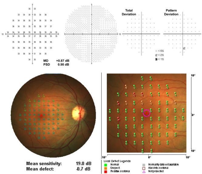
This diagnostic composite compares visual field testing modalities for ophthalmology. The top row illustrates data from a Humphrey Field Analyzer (HFA) using a 10-2 pattern and SITA Standard strategy. It includes a numeric sensitivity grid (decibels), a grayscale plot, and 'Total Deviation' and 'Pattern Deviation' probability maps for detecting localized scotomas. Global indices such as Mean Deviation (MD) and Pattern Standard Deviation (PSD) are provided. The bottom row displays MP-1 microperimetry results, featuring a fundus photograph with an overlaid 10-2 testing grid. The fundus image shows the optic disc, macula, and retinal vasculature. The magnified view on the right categorizes individual test points by color: green for normal sensitivity, yellow for suspect, and red for relative scotoma, with a legend for local defect classifications. This comparison demonstrates the integration of functional perimetry data with structural retinal anatomy, useful for diagnosing and monitoring macular diseases and glaucoma.
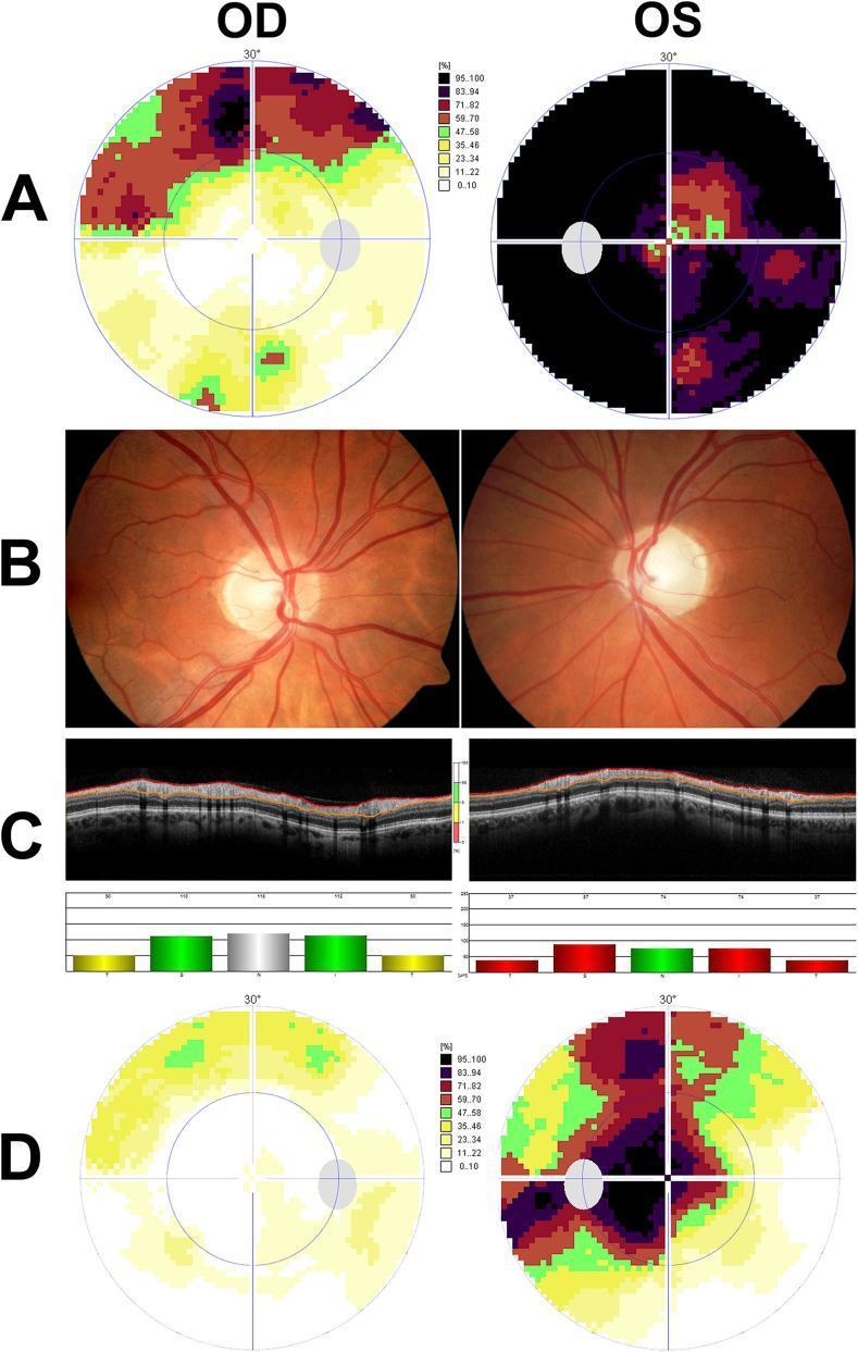
This composite educational graphic illustrates a neuro-ophthalmological workup for bilateral optic neuropathy. Panel A displays baseline threshold perimetry (visual field test) maps for the right (OD) and left eye (OS), showing an upper arcuate defect in the OD and profound, deep visual field loss in the OS. Panel B presents color fundus photographs; the right optic disc appears healthy, while the left optic disc demonstrates temporal pallor and mild cupping. Panel C shows peripapillary Optical Coherence Tomography (OCT) scans with associated Retinal Nerve Fiber Layer (RNFL) thickness bar graphs. The OD displays normal RNFL thickness (97 μm, green/yellow bars), whereas the OS shows significant pathological thinning (68 μm, red bars) falling below the reference range. Panel D displays follow-up threshold perimetry post-radiotherapy, indicating partial recovery of sensitivity in both eyes but with a persistent central scotoma in the left eye. These modalities collectively demonstrate the diagnosis and progression of optic nerve damage, relevant for clinical studies in neuro-oncology and ophthalmology.
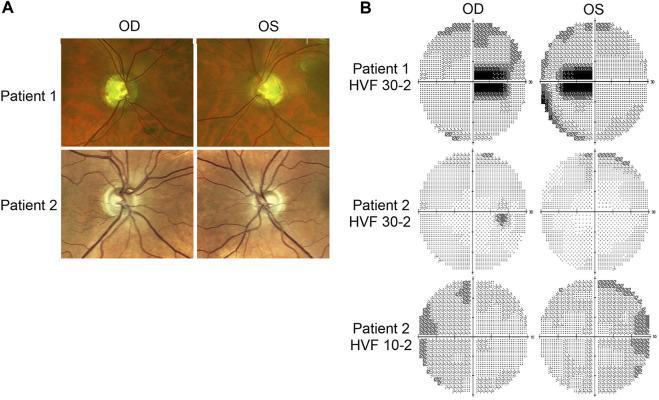
This composite educational graphic presents clinical ophthalmic diagnostic data for two patients, organized into two primary sections: fundus photography (A) and Humphrey Visual Field (HVF) testing (B). Panel A displays four fundus photographs showing the right (OD) and left (OS) eyes of two patients. Key clinical findings include bilateral temporal optic nerve head pallor, characteristic of hereditary optic neuropathies like Dominant Optic Atrophy (DOA). Patient 1 exhibits more extensive, yellowish-white pallor compared to the more localized temporal paleness in Patient 2. Panel B provides a series of perimetry reports (HVF 30-2 and 10-2). Patient 1's 30-2 tests demonstrate dense bilateral cecocentral scotomas, indicating significant loss of central vision sensitivity. Patient 2's 30-2 reports show much milder, scattered paracentral defects, while the more localized 10-2 test identifies superior temporal field loss within the central 10 degrees. This visualization illustrates the correlation between clinical optic nerve morphology (pallor) and functional visual field deficits in neuro-ophthalmology.
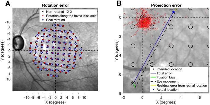
This figure illustrates the methodology for calculating rotation and projection errors in visual field (VF) perimetry using fundus imaging. Panel A shows a Spectralis fundus photograph overlaid with three different 10-2 mapping schemes centered on the fovea: a non-rotated grid (black points), a grid aligned to the fovea-disc axis (red points), and the actual observed retinal rotation from a Compass Microperimeter (empty blue circles). This demonstrates how anatomical variation affects the alignment of stimuli coordinates. Panel B provides a high-magnification view of a fundus-based coordinate system (in degrees) used to quantify projection errors. It distinguishes between intended test locations (empty black circles) and the actual stimulus location (blue dot). Visual markers represent different error components: a red dot cloud indicating fixation positions, a green line for fixation bias, a dashed black line for eye movement, and a yellow line for residual error from retinal rotation. The solid blue line connects the intended location to the actual projection, representing total error. This comparison is critical for structure-function analysis in ophthalmology, particularly for monitoring glaucoma progression.
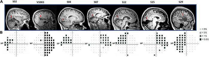
A composite figure correlating neuroanatomical lesions with functional visual field deficits in seven human subjects (labeled S02 through S29). Row A displays sagittal anatomical MRI brain scans for each subject. Red arrows indicate specific neuroanatomical lesions, including injuries to the primary visual cortex (V1), optic radiations, and temporoparietal regions, often resulting from historical ischemic or hemorrhagic strokes. Row B presents corresponding Humphrey perimetry test results (10-2 and 30-2 protocols) visualized as pattern deviation probability plots. These plots map visual field sensitivity across 10 to 30 degrees. Significant deficits, such as homonymous hemianopia and quadrantanopia, are indicated by dense clusters of black squares (probability p < 0.5%) and dotted squares (lower sensitivity). The visual data demonstrates the clinical correlation between focal cortical/subcortical brain damage and specific patterns of scotoma or visual field loss. This material is designed for advanced medical education in neurology, ophthalmology, and neuroimaging to illustrate the relationship between structural brain pathology and functional sensory impairment.
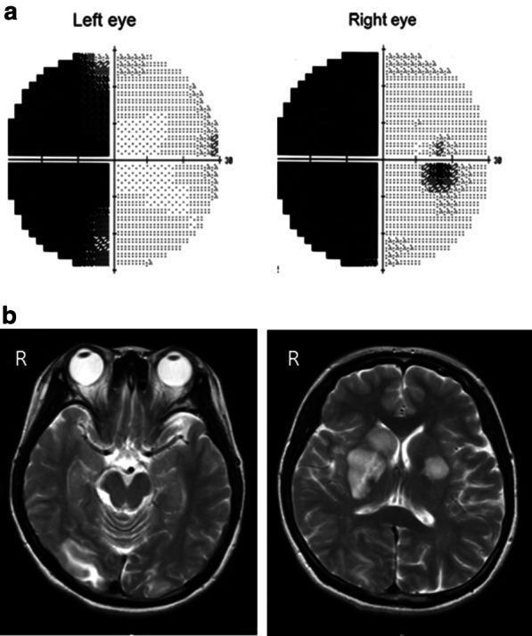
This composite educational image displays a correlation between clinical neuro-ophthalmology findings and neuroimaging. Section (a) shows Automated Static Perimetry (visual field tests) for the left and right eyes, exhibiting a dense left homonymous hemianopsia, characterized by total vision loss in the left temporal field of the left eye and left nasal field of the right eye. Section (b) provides two axial brain MRI slices using T1-weighted fluid-attenuated inversion recovery (T1-FLAIR) sequences. The images demonstrate areas of hyperintense signal indicating edema and infarction within the right basal ganglia (caudate and putamen) and the right occipital lobe. The occipital lesion specifically correlates with the functional visual field defect observed in section (a). This visual material is used to demonstrate the localization of intracranial pathology along the visual pathway, specifically post-chiasmatic lesions in the right hemisphere resulting in contralateral visual field deficits. It is relevant for medical training in neurology, ophthalmology, and radiology.
Goldmann perimeter visual field isopter scotoma
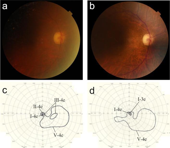
This composite educational graphic displays a comparison of ophthalmic findings for a right eye at two different time points. Panels (a) and (b) are color fundus photographs. Image (a) shows a hazy view of the posterior pole with poor definition of the optic nerve head and retinal vasculature, consistent with media opacity from endophthalmitis. Image (b) shows improved clarity at the final follow-up, revealing a clear optic disc and better visualization of the macula and retinal vessels. Panels (c) and (d) present Goldmann kinetic perimetry (visual field) results. Image (c) illustrates the initial visual field with multiple isopters (I-4e, II-4e, III-4e, and V-4e), showing a central scotoma and moderate peripheral constriction. Image (d) shows the final visual field with isopters I-4e, I-3e, and V-4e; while the III-4e isopter is absent and the field remains constricted, the overall sensitivity indicates functional preservation of vision. These images demonstrate the longitudinal management of glaucoma and infection, highlighting that despite complications like intraocular pressure fluctuations, key anatomical and functional markers were maintained.
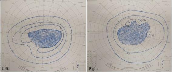
This diagnostic image consists of two Goldmann kinetic perimetry plots representing the left and right eyes of a patient. The plots map the functional integrity of the visual fields. Both eyes demonstrate a large, dense central scotoma, represented by prominent blue-shaded regions occupying the central fixation area. The left eye shows a relatively uniform, horizontally oval central defect. The right eye displays a more irregular central scotoma with adjacent satellite defects and notched borders. Concentric lines, or isopters, indicate the boundaries of peripheral vision for different stimulus intensities; both plots show marked concentric constriction, where the outermost isopters are significantly retracted toward the center compared to a normal physiological range. These findings are clinically significant for severe bilateral loss of central vision and peripheral field narrowing, characteristic of advanced Cancer-Associated Retinopathy (CAR). This visual material is used in ophthalmology and oncology to illustrate paraneoplastic syndromes affecting the retina and the resulting profound visual field deficits.
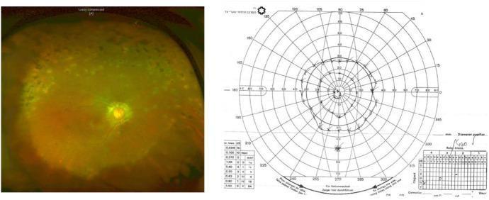
This composite educational figure consists of a pseudo-color ultra-widefield fundus photograph and a corresponding Goldmann visual field (GVF) kinetic perimetry chart of a right eye. The fundus image displays clear vitreous media and significant peripapillary scarring surrounding the optic nerve head. The peripheral retina shows diffuse, mottled hypo- and hyperpigmented choroidal lesions, characteristic of chronic inflammatory sequelae such as sympathetic ophthalmia. The GVF chart demonstrates severe concentric visual field constriction. Specifically, the outermost isopter at maximal light intensity (4dB) is restricted to approximately 30 degrees from the fovea, while a lower intensity stimulus (3dB) further constricts the perceived field to 20 degrees. This clinical pairing illustrates the correlation between peripheral retinochoroidal atrophy and significant functional visual loss, relevant for advanced ophthalmology education regarding uveitis complications and the assessment of permanent retinal damage.
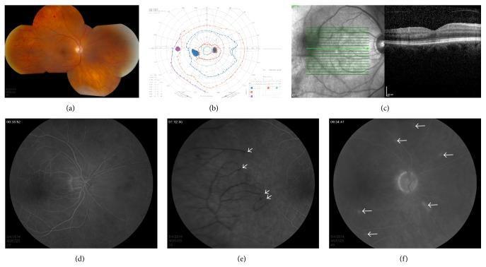
Multi-panel clinical diagnostic series illustrating ischemic hemorrhagic retinal vasculitis. Panel (a) is a color fundus montage showing significant arteriolar narrowing (attenuation), peripheral retinal pallor, and scattered dot-blot hemorrhages. Panel (b) depicts a Goldmann visual field with central isopter constriction, an enlarged blind spot, and a paracentral scotoma. Panel (c) provides a cross-sectional optical coherence tomography (OCT) scan showing preserved architecture of the retinal layers including the nerve fiber and photoreceptor layers. Panels (d–f) present a fluorescein angiography (FA) sequence: (d) illustrates delayed retinal and choroidal filling in the mid-phase; (e) demonstrates extensive late-phase peripheral capillary non-perfusion and terminal arteriolar occlusions (white arrows); (f) highlights scattered focal areas of vessel wall hyperfluorescence and leakage (white arrows). The findings are consistent with vancomycin-induced hemorrhagic occlusive retinal vasculitis (HORV) following intraocular surgery, focusing on severe peripheral ischemia despite a relatively normal posterior pole appearance on OCT.
PERIMETRY - Comprehensive Guide for MS Ophthalmology
PART 1: THEORY (Written Examination)
1. DEFINITION AND BASIC CONCEPTS
- 50° superiorly
- 60° nasally
- 70° inferiorly
- 90° temporally
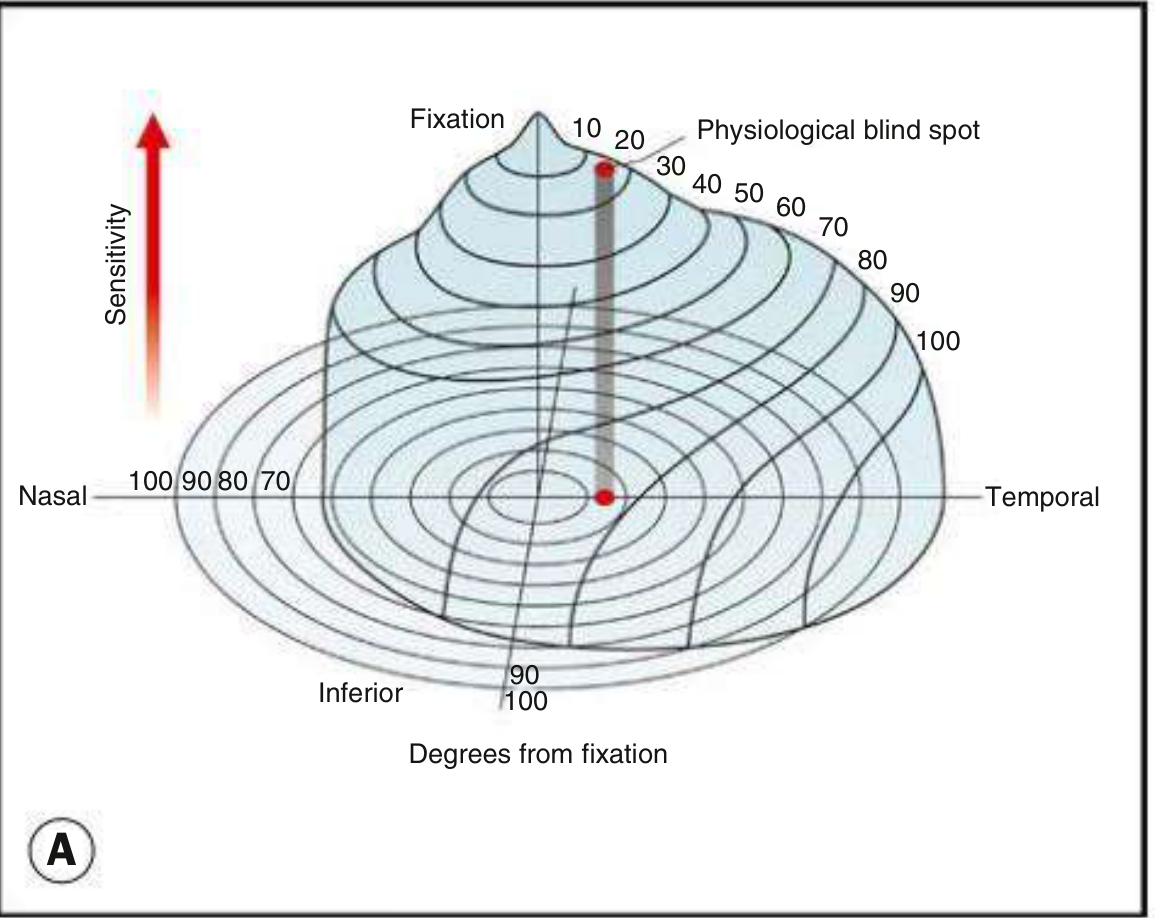
2. KEY DEFINITIONS (Must Know for Theory)
| Term | Definition |
|---|---|
| Isopter | A line connecting points of equal sensitivity on a 2D field chart; resembles contour lines on a map |
| Scotoma | An area of reduced (relative) or total (absolute) loss of vision surrounded by a seeing area |
| Threshold | The luminance of a stimulus at a given location which is perceived on 50% of presentations |
| Differential light sensitivity (DLS) | The degree by which luminance of a target must exceed background to be perceived |
| Luminance | Intensity/brightness of a light stimulus, measured in apostilbs (asb) |
| Decibels (dB) | Logarithmic unit used in perimetry; 10 dB = 1 log unit. Higher dB = higher retinal sensitivity |
| Mean sensitivity (MS) | Average sensitivity across all tested points |
| Suprathreshold | A stimulus intensity above threshold (definitely visible) |
- Sensitivity and stimulus intensity have an inverse relationship: higher dB = lower stimulus intensity = better retinal sensitivity
- The blind spot = 0 dB
- Normal foveal sensitivity ≈ 35 dB
- Normal sensitivity decreases by ~1 dB per 10 years after age 20
- The HFA uses a photopic background luminance of 31.5 asb (cone-mediated)
3. CLASSIFICATION OF PERIMETRY
A. By Stimulus Movement
- A stimulus of constant intensity is moved from a non-seeing to a seeing area
- The point at which it is first perceived is recorded
- Multiple meridians are tested with different stimulus intensities to plot isopters
- Goldmann perimetry is the standard kinetic method
- Also possible with automated perimeters (Humphrey/Octopus with kinetic software)
- The stimulus remains fixed in location; intensity is varied until it is detected (threshold found)
- More sensitive than kinetic for detecting subtle defects
- Usually automated
- Two subtypes:
- Threshold static - determines exact threshold at each point (more sensitive, longer)
- Suprathreshold static - tests each point using a set luminance (faster screening)
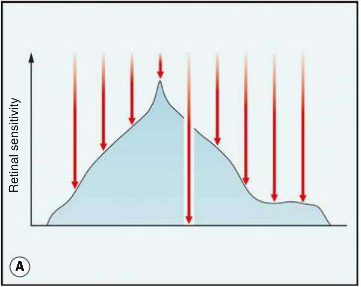
B. By Method of Administration
| Type | Details |
|---|---|
| Manual | Perimetrist presents stimuli manually; largely superseded but still used for cognitively limited patients and full peripheral field assessment |
| Automated | Computer-driven; reproducible, standardized; main clinical method |
4. GOLDMANN PERIMETRY (Manual Kinetic)
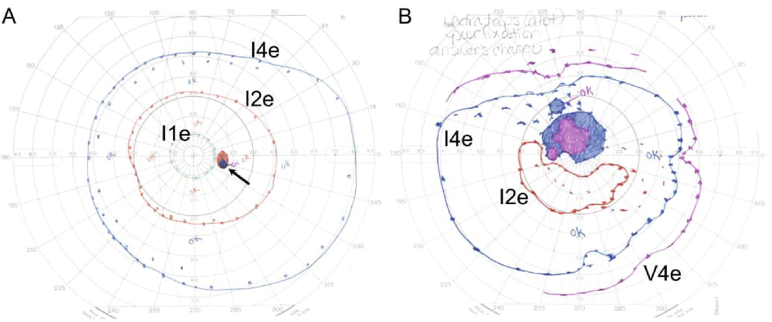
- Example: V4e = largest target (V), brightest luminance setting 4, no additional filter (e) - used for far peripheral field
- I2e - smaller, dimmer target used for central field
- I4e - medium target, intermediate brightness
- For central field: I2e, I1e
- For peripheral field: V4e, I4e
- Blind spot is routinely mapped with each test
- Maps the entire visual field including far periphery (>30°)
- Excellent for patients with poor central vision or inattention
- Exquisite topographic characterization
- Allows interaction between perimetrist and patient
- Better for neuro-ophthalmological conditions
- Requires a skilled, trained perimetrist
- Time-intensive
- Not easily reproduced or statistically compared between visits
- Operator-dependent variability
5. STANDARD AUTOMATED PERIMETRY (SAP) - Humphrey Field Analyzer (HFA)
Setup
- Patient places head in chin rest at center of a bowl-shaped perimeter
- Near refractive error is corrected with trial lenses
- Contralateral eye is occluded
- Patient maintains fixation on a central target and presses a handheld button when a stimulus is seen
- Background luminance: 31.5 asb (photopic)
- Maximum stimulus: 10,000 asb (Goldmann size III standard = 0.43°)
Testing Patterns (commonly tested)
| Pattern | Points Tested | Clinical Use |
|---|---|---|
| 24-2 | 54 points within central 24° | Standard for glaucoma, neurological |
| 30-2 | 76 points within central 30° | Neurological, neuro-ophthalmology |
| 10-2 | 68 points within central 10° | Advanced glaucoma, macular disease |
| Macula | Dense 4.2° pattern | Macular pathology |
| Esterman | Binocular strategy | Driving assessment |
Testing Strategies (Threshold Algorithms)
- Uses staircase method: stimuli presented in 4 dB steps, then 2 dB steps to "bracket" threshold
- Most accurate but time-consuming (~15 min/eye)
- SITA Standard - uses statistical modeling to estimate threshold; ~7 min/eye; comparable accuracy to FT
- SITA Fast - ~3-4 min/eye; less accurate, useful for unreliable patients
- SITA SWAP (Short Wavelength Automated Perimetry) - uses blue-on-yellow stimuli to test koniocellular pathway; detects early glaucomatous damage before SAP
- Three-zone strategy - points classified as normal, relatively depressed, or absolutely defective
- Faster, less detailed; used for mass screening
6. HUMPHREY FIELD ANALYZER PRINTOUT ANALYSIS
Step 1: Patient and Test Information
- Confirm: patient name, age, date, eye tested (OD/OS), corrective lens used
- Test type (e.g. SITA Standard 24-2), fixation target, background luminance
- Time taken, pupil size (must be ≥3 mm for reliable testing)
Step 2: Reliability Indices (Most Critical - Test them first!)
| Index | Acceptable Limit (SITA) | Acceptable Limit (Full Threshold) | Interpretation |
|---|---|---|---|
| Fixation Losses (FL) | <20% | <20% | Assessed by stimulating the blind spot; >20% = unreliable |
| False Positives (FP) | <15% | <33% | Patient pressing button without stimulus; printout looks unnaturally bright (pale grey scale) |
| False Negatives (FN) | <15% | <33% | Patient not responding to supra-threshold stimulus at known threshold; may indicate fatigue, inattention, or severe disease |
- High FP → grey scale printout appears abnormally pale (trigger-happy patient)
- High FN → grey scale printout shows a "clover-leaf" pattern (patient fatigue/inattention)
"If reliability indices are poor, visual field results cannot be meaningfully interpreted." - Kanski's Clinical Ophthalmology
Step 3: The Numerical Printout (Sensitivity Values)
- Each location in the visual field is assigned a dB value representing retinal sensitivity
- Normal foveal sensitivity: ~35 dB; normal peripheral sensitivity varies by eccentricity
- In full-threshold strategy, re-checked values are shown in brackets
Step 4: Grey Scale
- A graphical representation of the numerical data
- Darker areas = lower sensitivity
- Each shade change = approximately 5 dB
- Physiological blind spot = dark area in temporal paracentral field, ~15° from fixation
- Easy to see large defects but can obscure detail - always cross-reference with numerical values
- Beware: grey scale can be misleading if reliability is poor
Step 5: Total Deviation (TD) Map
- Shows the difference between the patient's measured threshold and the age-corrected normal value at each point
- Negative values = worse than normal; positive values = better than normal
- Not corrected for diffuse depression (e.g., from media opacity)
Step 6: Pattern Deviation (PD) Map
- Derived from TD values, but corrected for any generalized depression in the overall hill of vision
- Subtracts the most positive TD value (approximately the 85th percentile point)
- Reveals focal/localized defects that may be hidden by diffuse depression
- More useful in early glaucoma detection
- Less useful in severe diffuse loss
Step 7: Probability Plots (TD and PD)
- Each point is shown as a symbol representing the probability of abnormality:
- No symbol = P > 5% (normal)
- Light grey / small squares = P < 5%
- Medium squares = P < 2%
- Large dark squares = P < 1%
- Black = P < 0.5% (most abnormal)
- Darker symbols = higher probability of pathological significance
Step 8: Global Summary Indices
| Index | Definition | Normal | Clinical Significance |
|---|---|---|---|
| Mean Deviation (MD) | Average deviation from age-matched normal across all test points (weighted) | 0 to -2 dB | Negative = overall field depression; used for staging/monitoring |
| Pattern Standard Deviation (PSD) | Measure of variability/irregularity in the field relative to normal shape | <2 dB | Elevated PSD = focal loss; suppressed PSD in severe diffuse loss |
| Glaucoma Hemifield Test (GHT) | Compares mirror-image zones above and below horizontal midline | "Within Normal Limits" | Reports: Within NL / Borderline / Outside NL / Generalized Reduction / Abnormally High Sensitivity |
| Visual Field Index (VFI) | Percentage of normal VF; 100% = normal; 0% = complete loss | 100% | Used for progression analysis; less affected by cataract than MD |
- MS = Mean Sensitivity (equivalent to mean threshold, not deviation)
- MD = Mean Defect (equivalent to HFA Mean Deviation)
- SLV = Square root of Loss Variance (equivalent to PSD)
7. SOURCES OF ERROR IN PERIMETRY
Patient-Related
- Poor fixation - most important source of error
- Ptosis / dermatochalasis - causes superior field depression (artifact)
- Miosis - pupils <2 mm cause generalized depression; test at ≥3 mm, dilate if necessary
- Uncorrected refractive error - causes central/paracentral blur artifact
- Lens rim artifact - incorrect lens position creates a localized peripheral scotoma
- Learning effect - first field test often worse than subsequent ones
- Fatigue - especially with full-threshold strategies
- Inadequate dark adaptation - field worse if tested too soon after bright light
- Media opacities (cataract, corneal scar) - causes generalized sensitivity depression (mainly affects TD, less PD)
Instrument-Related
- Calibration errors
- Background luminance variation
- Fixation monitoring failures
8. SPECIAL TESTS IN PERIMETRY
Frequency Doubling Technology (FDT) Perimetry
- Uses a low spatial frequency grating that undergoes counter-phase flicker at high temporal frequency
- Stimulates the magnocellular (M-cell) pathway
- Detects glaucomatous damage earlier than SAP
- Quick, portable, useful as a screening tool
Short Wavelength Automated Perimetry (SWAP)
- Uses blue stimuli on a bright yellow background
- Tests the koniocellular (K-cell) pathway (small bistratified ganglion cells)
- Detects glaucomatous damage 3-5 years before conventional SAP
- More variable and affected by lens opacity
High Pass Resolution Perimetry (Ring Perimetry)
- Uses targets based on spatial resolution rather than light detection
- Tests midget ganglion cells
Flicker Perimetry / Temporal Modulation Perimetry
- Tests temporal contrast sensitivity
- Sensitive for early glaucoma and optic nerve disease
Multifocal Visual Evoked Potentials (mfVEP)
- Objective perimetry not dependent on patient response
- Useful in suspected non-organic visual loss
9. VISUAL FIELD DEFECTS AND THEIR LOCALIZATION
Pre-chiasmal Lesions (Retina / Optic Nerve)
| Defect | Lesion Site | Example Disease |
|---|---|---|
| Altitudinal defect (horizontal step) | Optic nerve / retina | AION, BRAO, Glaucoma (inferior arcuate) |
| Centrocecal scotoma | Optic nerve (papillomacular bundle) | Optic neuritis, toxic optic neuropathy, Leber's |
| Central scotoma | Macula or optic nerve | Macular degeneration, optic neuritis |
| Enlarged blind spot | Optic disc / peripapillary | Papilloedema, myopic optic disc |
| Arcuate defect (Bjerrum scotoma) | Optic nerve (arcuate fibres) | Glaucoma |
| Nasal step (Rönne step) | Superior or inferior nasal fibres | Glaucoma |
| Ring scotoma | Peripheral retina | Retinitis pigmentosa |
| Peripheral constriction | Entire retina | Advanced retinitis pigmentosa |
Chiasmal Lesions
| Defect | Mechanism | Example |
|---|---|---|
| Bitemporal hemianopia | Compression of crossing fibres (nasal fibres cross) | Pituitary adenoma, craniopharyngioma |
| Junctional scotoma | Compression at junction of optic nerve and chiasm; ipsilateral central scotoma + contralateral superior temporal defect | Pituitary adenoma, meningioma |
| Binasal hemianopia (rare) | Lateral chiasmal compression | Bilateral carotid aneurysms |
Post-chiasmal Lesions
| Defect | Lesion Site | Features |
|---|---|---|
| Homonymous hemianopia | Optic tract, LGN, optic radiation, occipital cortex | Affects both eyes on same side |
| Superior quadrantanopia | Temporal lobe (Meyer's loop) | "Pie in the sky" - temporal lobe lesion |
| Inferior quadrantanopia | Parietal lobe | "Pie on the floor" - parietal lobe lesion |
| Macular-sparing homonymous hemianopia | Occipital cortex | Posterior cerebral artery; macular representation at the "tip" of occipital lobe has dual blood supply |
| Congruous defects | More posterior (occipital cortex) | Identical in both eyes |
| Incongruous defects | More anterior (optic tract) | Different shape/size between eyes |
Key rule: The more posterior the post-chiasmal lesion, the more congruous the homonymous defect, and the more likely it is to show macular sparing.
10. GLAUCOMATOUS VISUAL FIELD DEFECTS (High Yield)
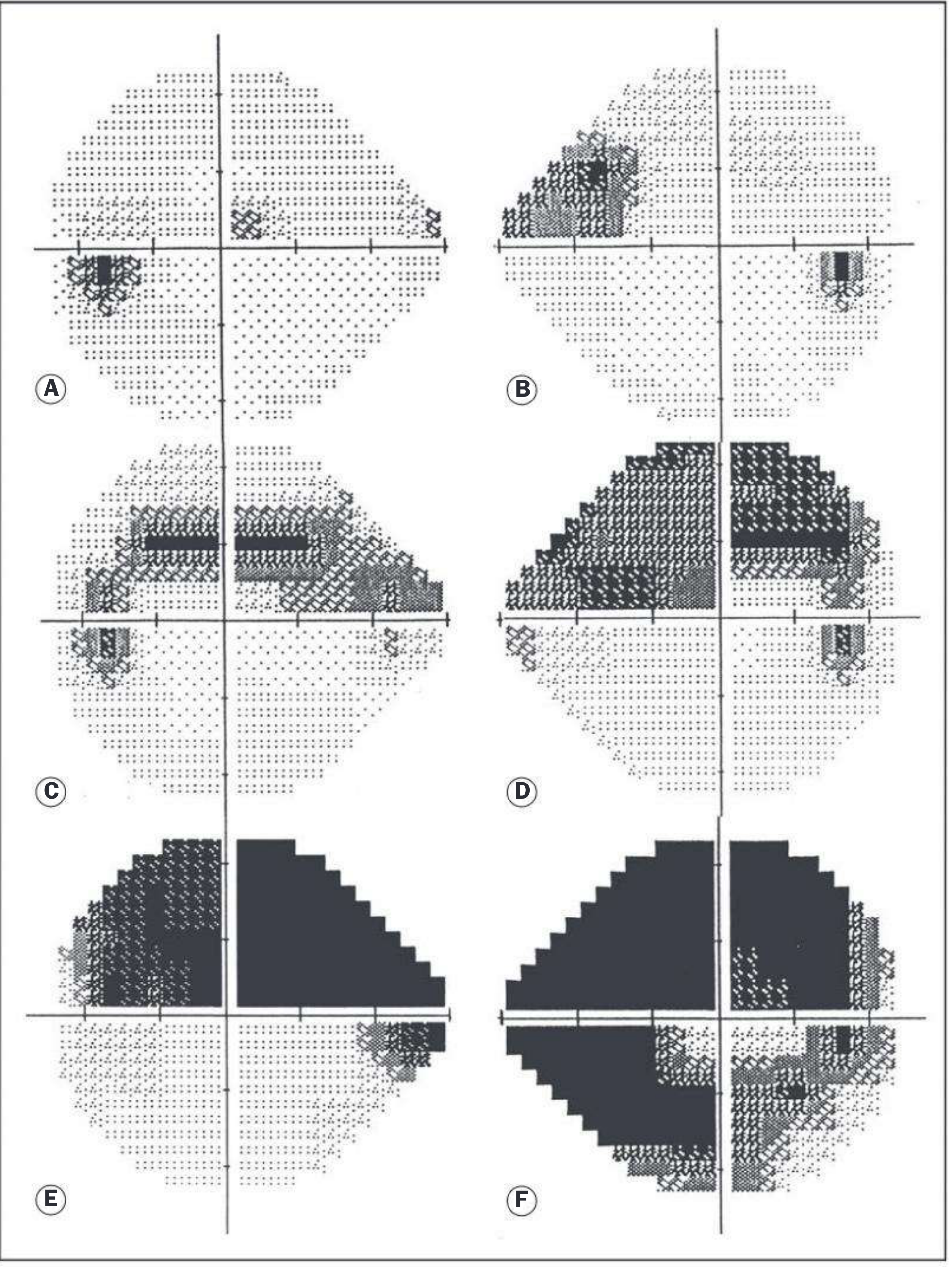
- Increased variability of threshold responses in areas that later develop defects
- Paracentral scotomas (small isolated depressions within 10-20° of fixation, often superonasally) - more common in Normal Tension Glaucoma (NTG)
- Nasal step (Rönne step): asymmetry above and below the horizontal meridian in the nasal field; bounded by the horizontal raphe
- Temporal wedge (rare, but similar significance)
- Arcuate defect (Bjerrum scotoma): between 10° and 20°, extends from the blind spot around fixation following the arcuate nerve fibre bundle
- Double arcuate / ring scotoma: superior and inferior arcuate defects merge
- End-stage: small central island + temporal island; use 10-2 pattern to monitor residual central field
- GHT outside normal limits on ≥2 consecutive occasions, OR
- A cluster of ≥3 non-edge points all depressed on PD at P <5%, with at least one at P <1%, on ≥2 consecutive occasions, OR
- Corrected PSD occurring in <5% of normal individuals on ≥2 consecutive fields
- Early: MD < -6 dB
- Moderate: MD -6 to -12 dB
- Advanced: MD > -12 dB
11. PROGRESSION ANALYSIS
- Annual deterioration in untreated glaucoma ≈ just over 1 dB MD/year (with significant individual variation)
- The HFA software's Guided Progression Analysis (GPA) uses event-based and trend-based analysis
- Compares each field to two baseline fields
- Flags "possible" and "likely" progression
- "Likely progression" requires consistent change on ≥3 consecutive fields
PART 2: PRACTICAL EXAMINATION
HOW TO PERFORM CONFRONTATION VISUAL FIELDS (Bedside/Practical)
Equipment
- No special equipment needed (hand/fingers as targets)
- Ideally use a red hat pin (5 mm red target) for central/colour comparison fields
Method: Finger Confrontation
- Sit directly opposite the patient at arm's length (~1 metre)
- Ask the patient to cover one eye; you cover your opposite eye (mirror image)
- Instruct the patient to maintain fixation on your nose throughout
- Compare your field with theirs (you serve as the control)
- Move a waggling finger from the periphery inward in each of the four quadrants
- Ask: "Can you see my finger moving? When does it appear?"
- Test the other eye
Method: Red Hat Pin (Central and Colour Fields)
- Hold a 5 mm red target at arm's length
- Ask if the patient can see the red colour
- Ask: "Does the red appear the same in both eyes? / In all parts of the field?"
- Compare colour desaturation across the vertical midline (nasal vs temporal)
- Test for central scotoma: bring target from periphery toward centre; does it disappear?
- Test for enlarged blind spot: move target from blind spot region outward
Confrontation - Specific Tests
- Hold up different numbers of fingers in each quadrant simultaneously or separately
- Ask patient to identify the number shown
- Present stimuli simultaneously in both hemifields
- Tests for visual inattention/extinction (a subtle hemianopia variant seen in parietal lesions)
- 10 × 10 cm grid with central fixation dot, held at 33 cm
- Assesses the central 10° (20° arc) in detail
- Ask: "Is the central dot visible? Are all four corners visible? Are any lines wavy, distorted, or missing?"
- Positive findings: metamorphopsia, central/paracentral scotoma, line distortion
- Key use: Macular disease (AMD, macular oedema), subtle central field loss
HOW TO PERFORM GOLDMANN PERIMETRY (Practical)
Pre-test Setup
- Confirm patient details; record the eye to be tested
- Explain the procedure clearly to the patient
- Correct refractive error using a trial frame (especially for >5D sphere or >3D cylinder)
- Cover the fellow eye with an eye patch
- Adjust chin rest so the eye is centered in the aperture
- Check pupil size (must be ≥3 mm; dilate with tropicamide if necessary)
- Ensure correct background illumination (1000 asb)
- Allow 5 minutes of dark adaptation in the perimetry room
Procedure
- Instruct the patient to fixate on the central target and respond immediately when a light is seen (oral response or button press)
- Map the blind spot first using the I4e stimulus - brings it in from different meridians to define the blind spot boundaries
- Test isopters from peripheral to central:
- Start with the large bright stimulus (V4e or I4e) for peripheral field
- Move to smaller dimmer stimuli (I2e, I1e) for central field
- Move the stimulus at a speed of ~2-3°/sec from the periphery inward
- Mark the point where the patient first responds
- Test at least 12-15 meridians per isopter (every 15-30°)
- Join the plotted points to draw the isopter
Interpreting the Goldmann Chart
- Uniform isopters = normal; each successive isopter should be smaller and more central
- Constricted isopters = peripheral field loss (e.g., retinitis pigmentosa, advanced glaucoma)
- Flattening/notching of an isopter = localized defect
- Central scotoma: all isopters are present peripherally but absent centrally (isopters don't close around fixation)
- Cecocentral scotoma: defect connecting the blind spot to the fixation area
- Non-organic fields: star/spiral shaped fields - the field should remain constant at a fixed testing distance; in non-organic disease, fields may "spiral" inward (getting smaller with repeated testing)
HOW TO PERFORM HFA AUTOMATED PERIMETRY (Practical)
Patient Preparation
- Record: name, date of birth, refraction, pupil size
- Place appropriate trial lens in the holder:
- Add +1.00 for patient >40 years (presbyopia correction based on working distance ~33 cm)
- Or use actual near addition required for test distance
- Note: high-power lenses and lens frames can cause rim artifacts
- Occlude fellow eye
- Adjust chin rest height (pupil centered in aperture)
- Demonstrate the test: play a practice run first
During the Test
- Monitor fixation via the Heijl-Krakau method (stimuli projected to the blind spot; if patient responds = fixation loss) or gaze tracker (plots eye position in real time below the printout)
- Remind the patient to maintain central fixation on the yellow target
- Instruct patient not to search but to press the button every time a flash of light is seen, even if faint
- Stop if patient is clearly fatigued; reschedule
Printout Interpretation - Step-by-step Practical Protocol
- Check date, age, eye (OD = right, OS = left), lens used, test strategy
- FL < 20%? FP < 15%? FN < 15% (SITA)?
- If any fail: unreliable test, interpret with extreme caution
- Dark areas = depressed areas
- Identify defect location: central, arcuate, nasal, altitudinal, hemianopic
- Remember: grey scale can look dramatic even in unreliable tests - always confirm with numerical values
- Look for numbers <20 dB (moderate depression), <10 dB (severe), 0 dB (absolute scotoma, shown as
<0) - A number in brackets = threshold was rechecked
- Look at the pattern of abnormal points (black squares)
- Assess whether depression is diffuse or focal
- This is often the most clinically useful: shows focal loss after correcting for any diffuse depression
- Focal loss on PD = likely pathological (glaucomatous, neurological)
- If diffuse depression on TD but PD is clean = likely media opacity (cataract) or pupil miosis
- MD: overall severity
- PSD: focality of defect
- GHT: hemifield asymmetry
- VFI: percentage remaining field
- "This is a reliable (FL/FP/FN all within limits) left eye automated field test using SITA Standard 24-2 strategy. It shows a superior arcuate defect corresponding to an inferior arcuate nerve fibre bundle defect, with a nasal step. GHT is outside normal limits. MD is -8.5 dB and PSD is elevated at 6.2 dB. The pattern deviation plot confirms the focal nature of the loss. These findings are consistent with moderate glaucomatous field loss."
COMMON PRACTICAL EXAM SCENARIOS
Case 1: Pituitary Adenoma
- Field: Bitemporal hemianopia (worse superiorly initially, as growing adenoma first compresses inferior chiasmal fibres from below)
- On HFA: Temporal field loss in both eyes, respecting the vertical midline
- On Goldmann: Isopters cut off at or near the vertical midline temporally in both eyes
Case 2: Glaucoma
- Field: Arcuate scotoma, nasal step, double arcuate, ring scotoma (late)
- On HFA: Focal loss on PD map, elevated PSD, abnormal GHT
- Staging: MD < -6 (early), -6 to -12 (moderate), > -12 (advanced)
Case 3: Retinitis Pigmentosa
- Field: Ring scotoma in mid periphery, progressive peripheral constriction; central island preserved until late
- On Goldmann: Peripheral isopters severely contracted; inner isopters (V4e) may form a ring-shaped defect
- On HFA: Only useful for monitoring central 24-30°; full extent needs Goldmann
Case 4: Optic Neuritis / Demyelination
- Field: Central scotoma, centrocecal scotoma, or diffuse depression
- MD: Significantly depressed
- PD: Central cluster of abnormal points
- Recovery: Field often improves after steroid treatment
Case 5: AION (Anterior Ischaemic Optic Neuropathy)
- Field: Altitudinal defect (commonly inferior altitudinal in arteritic AION due to superior disc ischaemia)
- Boundaries: Sharp horizontal meridian
Case 6: Non-organic (Functional) Visual Loss
- On Goldmann: Spiral/star-shaped field; constricted fields that do not expand with increasing testing distance (normal fields should enlarge with distance)
- On HFA: Scattered unreliable responses; high false positives and/or false negatives; inconsistent patterns
- Binocular kinetic perimetry may show crossed fields (non-physiological monocular constriction)
PRACTICAL EXAMINATION TIPS AND VIVA PEARLS
-
Always check reliability first before interpreting any HFA printout. State this aloud.
-
Goldmann stimulus notation: Know what Roman/Arabic numeral/letter means in the Goldmann system.
-
The physiological blind spot is at 15° temporal to fixation, slightly below the horizontal meridian, corresponding to the optic disc (no photoreceptors).
-
Pattern deviation vs Total deviation: PD corrects for diffuse depression; TD does not. In a cataract patient, TD may look terrible but PD will be relatively clean.
-
GHT significance: If GHT says "Outside Normal Limits," this is one of the HPA criteria for glaucomatous damage.
-
VFI vs MD: VFI is less affected by cataract and is preferred for monitoring glaucoma progression.
-
When to use Goldmann over HFA:
- Far peripheral field assessment (>30°)
- Patients who cannot cooperate with automated perimetry
- Very poor central vision (can't maintain fixation for HFA)
- Children, cognitively impaired patients
- Suspected non-organic visual loss
-
SITA Standard vs SITA Fast: SITA Standard is more accurate; SITA Fast is quicker but less precise. Use SITA Standard for most clinical decisions.
-
Learning effect: The first HFA field is often worse than subsequent ones. Ideally establish a baseline with 2 fields, then compare all subsequent tests to that baseline.
-
Artefacts to recognise on HFA:
- Peripheral ring of sensitivity loss = lens rim artefact (reposition trial lens)
- Superior field depression with normal inferior = ptosis/dermatochalasis (tape lid up and repeat)
- Generalised depression with clear PD = cataract or small pupil
- Clover-leaf pattern = false negatives (patient fatigue)
- Uniform pale grey scale = false positives (trigger-happy patient)
QUICK REVISION SUMMARY TABLE
| Feature | Goldmann | HFA SAP |
|---|---|---|
| Stimulus | Moving, constant intensity | Static, varying intensity |
| Field extent | Full (up to 90° temporal) | Central 24-30° (standard) |
| Background | 1000 asb | 31.5 asb |
| Operator | Perimetrist required | Automated |
| Reproducibility | Lower | Higher |
| Threshold | Estimated | Measured |
| Progression analysis | Difficult | Excellent (GPA, VFI) |
| Best for | Peripheral loss, neuro-ophthal, non-cooperative patients | Glaucoma monitoring, neurological field defects |
| Time | 20-30 min/eye | 6-8 min/eye (SITA Standard) |
Make it in pdf format
ls -la /tmp/workspace/ 2>/dev/null || mkdir -p /tmp/workspace && ls -la /tmp/workspace/
mkdir -p /tmp/workspace/perimetry-pdf
~/perimetry-pdf/generate_pdf.py
from reportlab.lib.pagesizes import A4
from reportlab.lib import colors
from reportlab.lib.styles import getSampleStyleSheet, ParagraphStyle
from reportlab.lib.units import cm, mm
from reportlab.platypus import (
SimpleDocTemplate, Paragraph, Spacer, Table, TableStyle,
HRFlowable, PageBreak, KeepTogether
)
from reportlab.lib.enums import TA_CENTER, TA_LEFT, TA_JUSTIFY
from reportlab.platypus import ListFlowable, ListItem
import urllib.request
import os
OUTPUT = "/tmp/workspace/perimetry-pdf/Perimetry_MS_Ophthalmology.pdf"
# ── colour palette ──────────────────────────────────────────────────
NAVY = colors.HexColor("#1a3a5c")
TEAL = colors.HexColor("#0d7377")
LIGHT_TEAL= colors.HexColor("#e8f7f8")
GOLD = colors.HexColor("#c8860a")
LIGHT_GOLD= colors.HexColor("#fdf6e3")
LIGHT_GREY= colors.HexColor("#f5f5f5")
MED_GREY = colors.HexColor("#888888")
RED_ACCENT= colors.HexColor("#c0392b")
WHITE = colors.white
BLACK = colors.black
# ── styles ───────────────────────────────────────────────────────────
base = getSampleStyleSheet()
def S(name, **kw):
"""Helper: clone base Normal and apply kwargs."""
s = ParagraphStyle(name, parent=base["Normal"], **kw)
return s
# Main title
TITLE_STYLE = S("DocTitle",
fontSize=26, textColor=WHITE, alignment=TA_CENTER,
spaceAfter=4, fontName="Helvetica-Bold", leading=32)
SUBTITLE_STYLE = S("DocSubtitle",
fontSize=13, textColor=colors.HexColor("#cce8ea"),
alignment=TA_CENTER, spaceAfter=2, fontName="Helvetica")
# Part header (PART 1 / PART 2)
PART_STYLE = S("PartHeader",
fontSize=14, textColor=WHITE, alignment=TA_CENTER,
fontName="Helvetica-Bold", spaceBefore=6, spaceAfter=6, leading=18)
# Section heading (##)
H1 = S("H1",
fontSize=14, textColor=WHITE, fontName="Helvetica-Bold",
spaceBefore=14, spaceAfter=4, leading=18)
# Sub-section heading (###)
H2 = S("H2",
fontSize=12, textColor=NAVY, fontName="Helvetica-Bold",
spaceBefore=10, spaceAfter=3, leading=16,
borderPad=2)
# Sub-sub heading (####)
H3 = S("H3",
fontSize=11, textColor=TEAL, fontName="Helvetica-Bold",
spaceBefore=7, spaceAfter=2, leading=14)
# Body text
BODY = S("Body",
fontSize=10, textColor=BLACK, fontName="Helvetica",
spaceBefore=2, spaceAfter=4, leading=15, alignment=TA_JUSTIFY)
# Bullet body
BULLET = S("Bullet",
fontSize=10, textColor=BLACK, fontName="Helvetica",
spaceBefore=1, spaceAfter=1, leading=14,
leftIndent=14, bulletIndent=4)
# Pearl box text
PEARL = S("Pearl",
fontSize=10, textColor=colors.HexColor("#7b3f00"),
fontName="Helvetica-BoldOblique",
spaceBefore=2, spaceAfter=2, leading=14,
leftIndent=8)
# Caption
CAPTION = S("Caption",
fontSize=8.5, textColor=MED_GREY, fontName="Helvetica-Oblique",
alignment=TA_CENTER, spaceAfter=6)
# Source line at bottom of page
SOURCE = S("Source",
fontSize=8, textColor=MED_GREY, fontName="Helvetica-Oblique",
alignment=TA_CENTER)
# ── helper flowables ─────────────────────────────────────────────────
def h1_block(text):
"""Full-width dark navy banner for section headings."""
tbl = Table([[Paragraph(text, H1)]], colWidths=[17*cm])
tbl.setStyle(TableStyle([
("BACKGROUND", (0,0), (-1,-1), NAVY),
("TOPPADDING", (0,0), (-1,-1), 7),
("BOTTOMPADDING", (0,0), (-1,-1), 7),
("LEFTPADDING", (0,0), (-1,-1), 10),
("RIGHTPADDING", (0,0), (-1,-1), 10),
("ROUNDEDCORNERS", [4]),
]))
return tbl
def h2_block(text):
return Paragraph(text, H2)
def h3_block(text):
return Paragraph(text, H3)
def body(text):
return Paragraph(text, BODY)
def bullet_list(items):
paras = []
for item in items:
paras.append(Paragraph(f"• {item}", BULLET))
return paras
def pearl_box(text):
inner = Paragraph(f"💡 {text}", PEARL)
tbl = Table([[inner]], colWidths=[17*cm])
tbl.setStyle(TableStyle([
("BACKGROUND", (0,0), (-1,-1), LIGHT_GOLD),
("TOPPADDING", (0,0), (-1,-1), 7),
("BOTTOMPADDING", (0,0), (-1,-1), 7),
("LEFTPADDING", (0,0), (-1,-1), 10),
("RIGHTPADDING", (0,0), (-1,-1), 10),
("BOX", (0,0), (-1,-1), 1, GOLD),
]))
return tbl
def tip_box(text):
inner = Paragraph(f"<b>TIP:</b> {text}", S("TipInner",
parent=base["Normal"], fontSize=10,
textColor=colors.HexColor("#155724"), fontName="Helvetica"))
tbl = Table([[inner]], colWidths=[17*cm])
tbl.setStyle(TableStyle([
("BACKGROUND", (0,0), (-1,-1), colors.HexColor("#d4edda")),
("TOPPADDING", (0,0), (-1,-1), 6),
("BOTTOMPADDING", (0,0), (-1,-1), 6),
("LEFTPADDING", (0,0), (-1,-1), 10),
("RIGHTPADDING", (0,0), (-1,-1), 10),
("BOX", (0,0), (-1,-1), 1, colors.HexColor("#28a745")),
]))
return tbl
def warn_box(text):
inner = Paragraph(f"<b>⚠ CAUTION:</b> {text}", S("WarnInner",
parent=base["Normal"], fontSize=10,
textColor=colors.HexColor("#721c24"), fontName="Helvetica"))
tbl = Table([[inner]], colWidths=[17*cm])
tbl.setStyle(TableStyle([
("BACKGROUND", (0,0), (-1,-1), colors.HexColor("#f8d7da")),
("TOPPADDING", (0,0), (-1,-1), 6),
("BOTTOMPADDING", (0,0), (-1,-1), 6),
("LEFTPADDING", (0,0), (-1,-1), 10),
("RIGHTPADDING", (0,0), (-1,-1), 10),
("BOX", (0,0), (-1,-1), 1, colors.HexColor("#f5c6cb")),
]))
return tbl
def divider():
return HRFlowable(width="100%", thickness=1, color=colors.HexColor("#dddddd"),
spaceAfter=6, spaceBefore=4)
def part_banner(text):
tbl = Table([[Paragraph(text, PART_STYLE)]], colWidths=[17*cm])
tbl.setStyle(TableStyle([
("BACKGROUND", (0,0), (-1,-1), TEAL),
("TOPPADDING", (0,0), (-1,-1), 10),
("BOTTOMPADDING", (0,0), (-1,-1), 10),
("LEFTPADDING", (0,0), (-1,-1), 10),
("RIGHTPADDING", (0,0), (-1,-1), 10),
]))
return tbl
def make_table(headers, rows, col_widths=None, alt_rows=True):
"""Build a styled table."""
head_style = S("TH", parent=base["Normal"],
fontSize=9.5, textColor=WHITE, fontName="Helvetica-Bold",
alignment=TA_CENTER)
cell_style = S("TD", parent=base["Normal"],
fontSize=9, textColor=BLACK, fontName="Helvetica",
alignment=TA_LEFT, leading=13)
data = [[Paragraph(h, head_style) for h in headers]]
for row in rows:
data.append([Paragraph(str(c), cell_style) for c in row])
if col_widths is None:
col_widths = [17*cm / len(headers)] * len(headers)
tbl = Table(data, colWidths=col_widths, repeatRows=1)
style = [
("BACKGROUND", (0,0), (-1,0), NAVY),
("ROWBACKGROUNDS", (0,1), (-1,-1), [LIGHT_GREY, WHITE] if alt_rows else [WHITE]),
("GRID", (0,0), (-1,-1), 0.4, colors.HexColor("#cccccc")),
("TOPPADDING", (0,0), (-1,-1), 5),
("BOTTOMPADDING", (0,0), (-1,-1), 5),
("LEFTPADDING", (0,0), (-1,-1), 6),
("RIGHTPADDING", (0,0), (-1,-1), 6),
("VALIGN", (0,0), (-1,-1), "TOP"),
]
tbl.setStyle(TableStyle(style))
return tbl
# ── cover page ────────────────────────────────────────────────────────
def cover_page():
elems = []
# Big title block
title_data = [[
Paragraph("PERIMETRY", TITLE_STYLE),
]]
title_tbl = Table(title_data, colWidths=[17*cm])
title_tbl.setStyle(TableStyle([
("BACKGROUND", (0,0), (-1,-1), NAVY),
("TOPPADDING", (0,0), (-1,-1), 30),
("BOTTOMPADDING", (0,0), (-1,-1), 10),
("LEFTPADDING", (0,0), (-1,-1), 20),
("RIGHTPADDING", (0,0), (-1,-1), 20),
]))
elems.append(Spacer(1, 2.5*cm))
elems.append(title_tbl)
subtitle_data = [[Paragraph(
"Comprehensive Guide for MS Ophthalmology<br/>Theory & Practical Examination",
SUBTITLE_STYLE)]]
sub_tbl = Table(subtitle_data, colWidths=[17*cm])
sub_tbl.setStyle(TableStyle([
("BACKGROUND", (0,0), (-1,-1), TEAL),
("TOPPADDING", (0,0), (-1,-1), 14),
("BOTTOMPADDING", (0,0), (-1,-1), 14),
("LEFTPADDING", (0,0), (-1,-1), 20),
("RIGHTPADDING", (0,0), (-1,-1), 20),
]))
elems.append(sub_tbl)
elems.append(Spacer(1, 1*cm))
# Quick-reference index
toc_items = [
("PART 1 — THEORY", [
"1. Definition & Basic Concepts",
"2. Key Definitions",
"3. Classification of Perimetry",
"4. Goldmann Perimetry",
"5. Standard Automated Perimetry (HFA)",
"6. HFA Printout Analysis",
"7. Sources of Error",
"8. Special Tests",
"9. Visual Field Defects & Localisation",
"10. Glaucomatous Field Defects",
"11. Progression Analysis",
]),
("PART 2 — PRACTICAL", [
"12. Confrontation Visual Fields",
"13. Goldmann Perimetry — Technique",
"14. HFA Automated Perimetry — Technique",
"15. Common Exam Scenarios",
"16. Practical Tips & Viva Pearls",
"17. Quick Revision Summary",
]),
]
for part, items in toc_items:
part_p = Paragraph(part, S("TOCPart", parent=base["Normal"],
fontSize=11, textColor=NAVY, fontName="Helvetica-Bold",
spaceBefore=8, spaceAfter=3))
elems.append(part_p)
for item in items:
elems.append(Paragraph(f" • {item}",
S("TOCItem", parent=base["Normal"],
fontSize=10, fontName="Helvetica",
spaceBefore=1, spaceAfter=1, textColor=BLACK)))
elems.append(Spacer(1, 1*cm))
elems.append(Paragraph(
"Sources: Kanski's Clinical Ophthalmology 10th Ed | Bradley & Daroff's Neurology in Clinical Practice | Guyton & Hall Physiology",
SOURCE))
elems.append(PageBreak())
return elems
# ── PART 1 CONTENT ────────────────────────────────────────────────────
def part1():
E = []
E.append(part_banner("PART 1 — THEORY (Written Examination)"))
E.append(Spacer(1, 6))
# ── Section 1
E.append(h1_block("1. DEFINITION AND BASIC CONCEPTS"))
E.append(Spacer(1, 4))
E.append(body(
"<b>Perimetry</b> is the systematic measurement of <b>differential light sensitivity</b> throughout the "
"visual field. It maps the 'island of vision' — the three-dimensional representation of visual "
"sensitivity across the entire visual field."))
E.append(Spacer(1, 4))
E.append(h3_block("Extent of the Normal Visual Field"))
E.append(make_table(
["Direction", "Extent"],
[["Superior", "~50°"], ["Nasal", "~60°"], ["Inferior", "~70°"], ["Temporal", "~90°"]],
col_widths=[8.5*cm, 8.5*cm]
))
E.append(Spacer(1, 4))
E.append(body(
"The peak of the hill corresponds to the <b>fovea</b> (highest sensitivity). "
"The <b>physiological blind spot</b> ('bottomless pit') lies temporally between 10° and 20°, "
"slightly below the horizontal meridian, corresponding to the optic disc (no photoreceptors)."))
E.append(Spacer(1, 4))
E.append(pearl_box(
"The nasal slope of the hill of vision is steeper than the temporal slope — reflecting the "
"asymmetric distribution of retinal ganglion cells."))
E.append(Spacer(1, 8))
# ── Section 2
E.append(h1_block("2. KEY DEFINITIONS"))
E.append(Spacer(1, 4))
E.append(make_table(
["Term", "Definition"],
[
["Isopter", "A line connecting points of equal sensitivity; encloses an area within which a stimulus of a given strength is visible. Resembles contour lines on a topographic map."],
["Scotoma", "An area of reduced ('relative') or total ('absolute') loss of vision surrounded by a seeing area."],
["Threshold", "The luminance of a stimulus at a given location which is perceived on 50% of presentations."],
["Differential Light Sensitivity (DLS)", "The degree by which luminance of a target must exceed background luminance to be perceived."],
["Luminance", "Intensity/brightness of a light stimulus, measured in apostilbs (asb). Higher asb = brighter."],
["Decibels (dB)", "Logarithmic unit. 10 dB = 1 log unit. Higher dB = higher retinal sensitivity (INVERSE to stimulus intensity)."],
["Mean Sensitivity (MS)", "Average sensitivity across all tested points."],
["Suprathreshold", "A stimulus intensity above threshold — definitely visible."],
["Background luminance", "Sets retinal adaptation state. HFA uses 31.5 asb (photopic). Goldmann uses 1000 asb."],
],
col_widths=[5*cm, 12*cm]
))
E.append(Spacer(1, 4))
E.append(h3_block("Decibel Scale — Critical Concept"))
E.extend(bullet_list([
"Sensitivity (dB) is INVERSELY related to stimulus intensity (asb)",
"Higher dB = lower stimulus needed = better retinal sensitivity",
"Blind spot = 0 dB | Normal fovea ≈ 35 dB | Normal periphery 15–30 dB",
"Sensitivity decreases by ~1 dB per 10 years after age 20",
"HFA uses photopic background (31.5 asb) — predominantly cone-mediated",
]))
E.append(Spacer(1, 8))
# ── Section 3
E.append(h1_block("3. CLASSIFICATION OF PERIMETRY"))
E.append(Spacer(1, 4))
E.append(h2_block("A. By Stimulus Movement"))
E.append(h3_block("1. Kinetic (Dynamic) Perimetry"))
E.extend(bullet_list([
"A stimulus of <b>constant intensity</b> is moved from a non-seeing to a seeing area",
"The point of first perception is recorded for multiple meridians",
"Multiple stimulus intensities are used to plot successive <b>isopters</b>",
"Standard instrument: <b>Goldmann perimeter</b> (manual); also possible with automated perimeters",
"Best for: full peripheral field, neuro-ophthalmology, non-cooperative patients",
]))
E.append(Spacer(1, 4))
E.append(h3_block("2. Static Perimetry"))
E.extend(bullet_list([
"Stimulus <b>location is fixed</b>; intensity is varied until threshold is reached",
"More sensitive than kinetic for detecting subtle defects",
"Usually automated (HFA, Octopus)",
"<b>Threshold static:</b> determines exact dB threshold at each point — most accurate",
"<b>Suprathreshold static:</b> tests with a set luminance — faster, screening only",
]))
E.append(Spacer(1, 6))
E.append(h2_block("B. By Method of Administration"))
E.append(make_table(
["Type", "Details", "Current Use"],
[
["Manual", "Perimetrist presents stimuli by hand; patient gives verbal/motor response", "Limited — cognitively impaired patients, peripheral field assessment"],
["Automated (SAP)", "Computer-driven; reproducible, standardized stimuli; statistical analysis", "Routine clinical standard"],
],
col_widths=[3.5*cm, 8*cm, 5.5*cm]
))
E.append(Spacer(1, 8))
# ── Section 4
E.append(h1_block("4. GOLDMANN PERIMETRY (Manual Kinetic)"))
E.append(Spacer(1, 4))
E.append(h2_block("Design & Specifications"))
E.extend(bullet_list([
"Hemispherical white bowl — background illumination: <b>1000 asb</b> (mesopic)",
"Examiner operates the instrument and records patient responses manually",
"Invented by Hans Goldmann in <b>1945</b>",
]))
E.append(Spacer(1, 6))
E.append(h2_block("Stimulus Notation (Must Memorise)"))
E.append(make_table(
["Component", "Notation", "Description"],
[
["Target Size", "Roman numeral I–V", "I = smallest (1/16 mm²); V = largest (64 mm²)"],
["Luminance Filter", "Arabic numeral 1–4", "4 = brightest (no filter)"],
["Additional Filter", "Lowercase letter a–e", "e = no additional attenuation (brightest); a = most attenuated"],
["Example: V4e", "Largest size, highest luminance, no filter", "Used for full peripheral field mapping"],
["Example: I2e", "Smallest size, medium luminance", "Used for central field, small scotomas"],
["Example: I4e", "Smallest size, maximum luminance", "Standard central field isopter"],
],
col_widths=[3.5*cm, 5.5*cm, 8*cm]
))
E.append(Spacer(1, 6))
E.append(h2_block("Advantages vs Disadvantages"))
E.append(make_table(
["Advantages", "Disadvantages"],
[
["Maps FULL visual field (up to 90° temporal)", "Requires skilled, trained perimetrist"],
["Excellent for patients with poor central vision", "Time-intensive (~20–30 min/eye)"],
["Interactive — perimetrist can adapt to patient", "Operator-dependent variability"],
["Superior for peripheral & neurological assessment", "Not easily compared statistically over time"],
["Best for suspected non-organic visual loss", "Being replaced by automated methods in many centres"],
],
col_widths=[8.5*cm, 8.5*cm]
))
E.append(Spacer(1, 8))
# ── Section 5
E.append(h1_block("5. STANDARD AUTOMATED PERIMETRY (HFA)"))
E.append(Spacer(1, 4))
E.append(body(
"<b>Standard Automated Perimetry (SAP)</b> is the routine clinical method. "
"The <b>Humphrey Field Analyzer (HFA; Carl Zeiss)</b> and <b>Octopus (Haag-Streit)</b> are the most widely used. "
"Background luminance: 31.5 asb (photopic). Maximum stimulus: 10,000 asb. "
"Standard target: <b>Goldmann size III</b> (0.43°)."))
E.append(Spacer(1, 6))
E.append(h2_block("Testing Patterns"))
E.append(make_table(
["Pattern", "Points Tested", "Field Extent", "Clinical Use"],
[
["24-2", "54 points", "Central 24°", "Standard for glaucoma, neurological"],
["30-2", "76 points", "Central 30°", "Neurological, neuro-ophthalmology"],
["10-2", "68 points", "Central 10°", "Advanced glaucoma, macular disease"],
["Macula", "Dense grid", "Central 4.2°", "Macular pathology"],
["Esterman", "Binocular", "Full binocular", "Driving assessment"],
],
col_widths=[2.5*cm, 3*cm, 3*cm, 8.5*cm]
))
E.append(Spacer(1, 6))
E.append(h2_block("Testing Strategies"))
E.append(make_table(
["Strategy", "Method", "Duration", "Notes"],
[
["Full Threshold (FT)", "4 dB then 2 dB staircase to bracket threshold", "~15 min/eye", "Most accurate; gold standard"],
["SITA Standard", "Statistical modelling; adaptive algorithm", "~7 min/eye", "Clinical standard; accuracy ≈ FT"],
["SITA Fast", "Faster variant of SITA", "~3–4 min/eye", "Less accurate; for unreliable/elderly"],
["SITA SWAP", "Blue stimulus on yellow background", "~8 min/eye", "Tests koniocellular path; detects early glaucoma"],
["Suprathreshold", "Fixed suprathreshold stimulus at each point", "~3 min/eye", "Screening only; misses subtle defects"],
],
col_widths=[3*cm, 5*cm, 3*cm, 6*cm]
))
E.append(Spacer(1, 8))
# ── Section 6
E.append(h1_block("6. HFA PRINTOUT ANALYSIS"))
E.append(Spacer(1, 4))
E.append(pearl_box(
"In ALL exams — check RELIABILITY INDICES first before interpreting any HFA printout. "
"An unreliable test cannot be meaningfully interpreted."))
E.append(Spacer(1, 6))
E.append(h2_block("Step 1: Patient & Test Information"))
E.extend(bullet_list([
"Confirm: patient name, age, date, eye (OD = right, OS = left)",
"Test type (e.g. SITA Standard 24-2), corrective lens used, pupil size (must be ≥3 mm)",
"Time taken, fixation target, background luminance",
]))
E.append(h2_block("Step 2: Reliability Indices"))
E.append(make_table(
["Index", "SITA Limit", "Full Threshold Limit", "Interpretation"],
[
["Fixation Losses (FL)", "<20%", "<20%", "Stimuli projected to blind spot; response = patient moved eye. High FL = poor fixation"],
["False Positives (FP)", "<15%", "<33%", "Response without stimulus. High FP = unreliable; grey scale appears PALE"],
["False Negatives (FN)", "<15%", "<33%", "No response to supra-threshold stimulus. High FN = fatigue/inattention; grey scale shows CLOVER-LEAF pattern"],
],
col_widths=[3*cm, 2.5*cm, 3*cm, 8.5*cm]
))
E.append(Spacer(1, 4))
E.append(make_table(
["Pattern on Printout", "Reliability Issue"],
[
["Abnormally PALE grey scale", "High False Positives (trigger-happy patient)"],
["CLOVER-LEAF grey scale", "High False Negatives (fatigued/inattentive patient)"],
["Scattered, random defects", "Poor fixation OR genuinely unreliable responses"],
],
col_widths=[8.5*cm, 8.5*cm]
))
E.append(Spacer(1, 6))
E.append(h2_block("Step 3: Numerical Display (Sensitivity Values)"))
E.extend(bullet_list([
"Each location shows measured/estimated threshold in <b>dB</b>",
"Numbers in <b>brackets</b> = threshold was re-checked (unexpected >5 dB result)",
"Values <20 dB = moderate depression; <10 dB = severe; '0' or '<0' = absolute scotoma",
"Normal foveal sensitivity ≈ 35 dB; decreases with eccentricity",
]))
E.append(h2_block("Step 4: Grey Scale"))
E.extend(bullet_list([
"Graphical representation: <b>darker = lower sensitivity</b>",
"Each shade change ≈ 5 dB",
"Physiological blind spot = dark area ~15° temporal to fixation, slightly below horizontal",
"Easy for large defects; can be misleading in unreliable tests — always cross-reference with numbers",
]))
E.append(h2_block("Step 5: Total Deviation (TD) Map"))
E.extend(bullet_list([
"Difference between patient's threshold and the <b>age-corrected normal</b> at each point",
"Negative values = worse than normal; positive = better than normal",
"<b>Not</b> corrected for diffuse depression (e.g. from cataract)",
"Shows BOTH focal and diffuse loss",
]))
E.append(h2_block("Step 6: Pattern Deviation (PD) Map"))
E.extend(bullet_list([
"TD values corrected for any <b>generalised depression</b> in the overall field",
"Subtracts the ~85th percentile point — reveals FOCAL/LOCALISED defects",
"Most useful for detecting early glaucomatous loss",
"If TD is depressed but PD is clean → likely <b>media opacity (cataract) or miosis</b>",
"Less useful when there is severe diffuse loss",
]))
E.append(h2_block("Step 7: Probability Plots (TD and PD)"))
E.append(make_table(
["Symbol", "Probability of Abnormality"],
[
["No symbol (blank)", "P > 5% — within normal range"],
["Light grey / small square", "P < 5%"],
["Medium square", "P < 2%"],
["Large square", "P < 1%"],
["Solid black square", "P < 0.5% — highly significant"],
],
col_widths=[8.5*cm, 8.5*cm]
))
E.append(h2_block("Step 8: Global Summary Indices"))
E.append(make_table(
["Index", "Definition", "Normal", "Clinical Use"],
[
["Mean Deviation (MD)", "Weighted average deviation from age-matched normal across all points", "0 to –2 dB", "Overall severity; staging glaucoma; monitoring"],
["Pattern Standard Deviation (PSD)", "Measure of variability/irregularity relative to normal field shape", "<2 dB", "Elevated = focal loss; suppressed in severe diffuse loss"],
["Glaucoma Hemifield Test (GHT)", "Compares mirror-image zones above and below horizontal midline", "Within Normal Limits", "Reports: Within NL / Borderline / Outside NL / Generalised Reduction / Abnormally High Sensitivity"],
["Visual Field Index (VFI)", "% of normal visual field remaining; 100% = normal; 0% = total loss", "100%", "Progression monitoring; less affected by cataract than MD"],
],
col_widths=[3*cm, 5.5*cm, 2.5*cm, 6*cm]
))
E.append(Spacer(1, 4))
E.append(h3_block("Octopus Equivalents"))
E.append(make_table(
["HFA Term", "Octopus Equivalent"],
[
["Mean Deviation (MD)", "Mean Defect (MD)"],
["Pattern Standard Deviation (PSD)", "Square Root of Loss Variance (SLV)"],
["Mean Sensitivity", "Mean Sensitivity (MS) — average threshold, not deviation"],
],
col_widths=[8.5*cm, 8.5*cm]
))
E.append(Spacer(1, 8))
# ── Section 7
E.append(h1_block("7. SOURCES OF ERROR IN PERIMETRY"))
E.append(Spacer(1, 4))
E.append(h2_block("Patient-Related Errors"))
E.append(make_table(
["Error Source", "Effect on Printout", "Solution"],
[
["Poor fixation", "Generalised scattered loss; high FL", "Remind patient; use gaze tracker; switch to kinetic"],
["Ptosis / Dermatochalasis", "Superior field depression (artefact)", "Tape lid up; repeat test"],
["Miosis (<2 mm pupil)", "Generalised sensitivity depression", "Dilate with tropicamide; record pupil size"],
["Uncorrected refractive error", "Central/paracentral blur artefact", "Correct with trial lens"],
["Lens rim artefact", "Peripheral ring scotoma", "Reposition trial lens"],
["Cataract / Media opacity", "Generalised TD depression; PD relatively clear", "Note on report; VFI preferred over MD"],
["Learning effect", "First test worse than subsequent", "Establish baseline with 2 fields before monitoring"],
["Fatigue", "High false negatives; clover-leaf pattern", "Use SITA Fast or suprathreshold; shorter test"],
["Inadequate adaptation", "Falsely depressed sensitivity", "Allow 5 min adaptation before testing"],
],
col_widths=[3.5*cm, 6.5*cm, 7*cm]
))
E.append(Spacer(1, 8))
# ── Section 8
E.append(h1_block("8. SPECIAL TESTS IN PERIMETRY"))
E.append(Spacer(1, 4))
E.append(make_table(
["Test", "Stimulus", "Pathway Tested", "Clinical Use"],
[
["Frequency Doubling Technology (FDT)", "Low spatial frequency grating with high-frequency counter-phase flicker", "Magnocellular (M-cell) pathway", "Early glaucoma screening; quick and portable"],
["SWAP (Short Wavelength Automated Perimetry)", "Blue stimulus on bright yellow background", "Koniocellular (K-cell) pathway — small bistratified ganglion cells", "Detects glaucoma 3–5 years before conventional SAP; affected by lens opacity"],
["High Pass Resolution Perimetry", "Ring targets based on spatial resolution", "Midget ganglion cells (P-cell)", "Early glaucomatous damage"],
["Flicker / Temporal Modulation Perimetry", "Flickering stimuli", "Temporal contrast sensitivity (M-cell)", "Early optic nerve disease, glaucoma"],
["Multifocal VEP (mfVEP)", "Flickering dartboard pattern; VEP recording", "Objective — no patient response required", "Non-organic visual loss, medicolegal, paediatric"],
["Microperimetry (MP-1, MAIA)", "Static stimuli on fundus image", "Focal macular sensitivity mapped to anatomy", "Macular degeneration, epiretinal membrane, myopic maculopathy"],
],
col_widths=[3.5*cm, 4*cm, 4.5*cm, 5*cm]
))
E.append(Spacer(1, 8))
# ── Section 9
E.append(PageBreak())
E.append(part_banner("VISUAL FIELD DEFECTS & LOCALISATION"))
E.append(Spacer(1, 6))
E.append(h1_block("9. VISUAL FIELD DEFECTS AND THEIR LOCALISATION"))
E.append(Spacer(1, 4))
E.append(h2_block("A. Pre-chiasmal Lesions (Retina / Optic Nerve)"))
E.append(make_table(
["Defect", "Lesion Site", "Example Disease"],
[
["Altitudinal defect (horizontal step)", "Optic nerve / retinal artery", "AION, BRAO, glaucoma (inferior arcuate)"],
["Centrocecal scotoma", "Optic nerve — papillomacular bundle", "Optic neuritis, toxic optic neuropathy, Leber's LHON"],
["Central scotoma", "Macula OR optic nerve", "Macular degeneration, optic neuritis"],
["Enlarged blind spot", "Optic disc / peripapillary region", "Papilloedema, myopic optic disc, optic disc drusen"],
["Arcuate defect (Bjerrum scotoma)", "Arcuate RNFL fibres at optic nerve head", "Glaucoma (most common)"],
["Nasal step (Rönne step)", "Superior or inferior nasal RNFL fibres", "Glaucoma"],
["Ring scotoma", "Mid-peripheral retina", "Retinitis pigmentosa"],
["Peripheral constriction", "Entire peripheral retina", "Advanced RP, advanced glaucoma"],
["Cecocentral scotoma", "Papillomacular bundle connecting disc to macula", "Toxic/nutritional optic neuropathy, LHON, optic neuritis"],
],
col_widths=[5*cm, 5.5*cm, 6.5*cm]
))
E.append(Spacer(1, 6))
E.append(h2_block("B. Chiasmal Lesions"))
E.append(make_table(
["Defect", "Mechanism", "Example Lesion"],
[
["Bitemporal hemianopia", "Compression of CROSSING nasal fibres at chiasm", "Pituitary adenoma (most common), craniopharyngioma"],
["Superior bitemporal defect first", "Inferior chiasmal fibres cross first; pressure from BELOW (adenoma)", "Pituitary macroadenoma"],
["Inferior bitemporal defect first", "Superior chiasmal fibres compressed first; pressure from ABOVE", "Craniopharyngioma, suprasellar meningioma"],
["Junctional scotoma (Traquair)", "Compression at junction of optic nerve & chiasm: ipsilateral central scotoma + contralateral superior temporal defect", "Pituitary adenoma, meningioma"],
["Binasal hemianopia (rare)", "Lateral chiasmal compression of non-crossing temporal fibres", "Bilateral carotid aneurysms, bilateral optic disc disease"],
],
col_widths=[4.5*cm, 7*cm, 5.5*cm]
))
E.append(Spacer(1, 6))
E.append(h2_block("C. Post-chiasmal Lesions"))
E.append(make_table(
["Defect", "Lesion Site", "Key Features"],
[
["Homonymous hemianopia", "Optic tract, LGN, optic radiation, or occipital cortex", "Affects same side in BOTH eyes"],
["Superior quadrantanopia ('pie in the sky')", "Temporal lobe — Meyer's loop (inferior fibres of optic radiation)", "Temporal lobe lesion; usually incongruous"],
["Inferior quadrantanopia ('pie on the floor')", "Parietal lobe (superior fibres of optic radiation)", "Parietal lobe lesion"],
["Macular-sparing homonymous hemianopia", "Occipital cortex (posterior cerebral artery territory)", "Macular cortex at tip of occipital lobe has dual blood supply; also patient scans toward hemianopic side"],
["Congruous homonymous defect", "More posterior (occipital cortex)", "Identical pattern in both eyes — more posterior lesion"],
["Incongruous homonymous defect", "More anterior (optic tract)", "Different size/shape in the two eyes — more anterior lesion"],
["Homonymous scotoma / quadrantanopia with macular sparing", "Occipital lobe with sparing of macular cortex", "Small cortical lesion; patient may be unaware"],
],
col_widths=[5*cm, 5*cm, 7*cm]
))
E.append(Spacer(1, 4))
E.append(pearl_box(
"Key Rule: The more POSTERIOR the post-chiasmal lesion, the more CONGRUOUS the defect "
"and the more likely it is to show MACULAR SPARING. "
"Optic tract lesions = incongruous; Occipital lesions = congruous with macular sparing."))
E.append(Spacer(1, 8))
# ── Section 10
E.append(h1_block("10. GLAUCOMATOUS VISUAL FIELD DEFECTS"))
E.append(Spacer(1, 4))
E.append(h2_block("Sequence of Glaucomatous Field Loss"))
E.append(make_table(
["Stage", "Field Finding", "Notes"],
[
["1 — Earliest", "Increased variability of threshold responses", "No visible defect yet; statistical measure only"],
["2 — Early", "Paracentral scotomas within 10–20° of fixation, often superonasally", "More common in Normal Tension Glaucoma (NTG)"],
["3 — Early-Moderate", "Nasal step (Rönne step): asymmetry above/below horizontal midline in nasal field", "Bounded by the horizontal raphe"],
["4 — Moderate", "Temporal wedge (less common)", "Similar significance to nasal step"],
["5 — Moderate", "Arcuate defect (Bjerrum scotoma): extends from blind spot around fixation", "Between 10–20° of fixation; follows arcuate RNFL bundle"],
["6 — Advanced", "Double arcuate / ring scotoma: superior + inferior arcuate defects merge", "Annular scotoma surrounding fixation"],
["7 — End-stage", "Small central island + temporal island", "Use 10-2 pattern; monitor VFI carefully"],
],
col_widths=[2.5*cm, 6*cm, 8.5*cm]
))
E.append(Spacer(1, 6))
E.append(h2_block("Hodapp-Parrish-Anderson (HPA) Criteria for Glaucomatous Damage on SAP"))
E.append(body("At least ONE of the following on TWO consecutive fields:"))
E.extend(bullet_list([
"GHT outside normal limits",
"A cluster of ≥3 non-edge points, all depressed on PD at P <5%, with at least one at P <1%",
"Corrected PSD occurring in <5% of normal individuals",
]))
E.append(Spacer(1, 4))
E.append(h2_block("Staging by Mean Deviation (MD)"))
E.append(make_table(
["Stage", "MD Value", "Clinical Features"],
[
["Early", "MD < –6 dB", "Subtle arcuate defects, nasal step; good central vision"],
["Moderate", "MD –6 to –12 dB", "Definite arcuate/ring scotoma; some central involvement"],
["Advanced", "MD > –12 dB", "Ring scotoma, small central island; significant disability"],
["End-stage", "MD > –20 dB", "Residual central and/or temporal island only"],
],
col_widths=[3*cm, 4*cm, 10*cm]
))
E.append(Spacer(1, 8))
# ── Section 11
E.append(h1_block("11. PROGRESSION ANALYSIS"))
E.append(Spacer(1, 4))
E.append(h2_block("Methods of Progression Detection"))
E.append(make_table(
["Method", "Description", "Tool"],
[
["Trend-based (linear regression)", "Linear regression of MD over time; rate = dB/year", "HFA Overview printout; manual calculation"],
["Event-based (GPA)", "Compares each field to two baseline fields; flags 'possible' and 'likely' progression", "Guided Progression Analysis (GPA) software on HFA"],
["Point-wise linear regression", "Regression at each test point individually; identifies locally progressing points", "PROGRESSOR software; Statpac on HFA"],
],
col_widths=[4*cm, 8*cm, 5*cm]
))
E.append(Spacer(1, 4))
E.extend(bullet_list([
"Annual deterioration in untreated glaucoma ≈ just over <b>1 dB MD/year</b> (wide individual variation)",
"'Likely progression' on GPA requires consistent change on <b>≥3 consecutive fields</b>",
"At least <b>2 baseline fields</b> should be obtained before monitoring begins",
"<b>VFI</b> is preferred over MD for progression monitoring as it is less affected by cataract",
"Rate of progression determines urgency of treatment escalation",
]))
E.append(Spacer(1, 8))
return E
# ── PART 2 CONTENT ────────────────────────────────────────────────────
def part2():
E = []
E.append(PageBreak())
E.append(part_banner("PART 2 — PRACTICAL EXAMINATION"))
E.append(Spacer(1, 6))
# ── Section 12
E.append(h1_block("12. CONFRONTATION VISUAL FIELDS (Bedside / OSCE)"))
E.append(Spacer(1, 4))
E.append(h2_block("Equipment"))
E.extend(bullet_list([
"No special equipment required for basic finger confrontation",
"Ideal: <b>5 mm red target (hat pin)</b> for central field, colour comparison, and scotoma testing",
"Amsler grid (10×10 cm, held at 33 cm) for central 10° assessment",
]))
E.append(Spacer(1, 6))
E.append(h2_block("Finger Confrontation — Step by Step"))
steps = [
"Sit directly opposite the patient at <b>arm's length (~1 metre)</b>",
"Ask the patient to cover ONE eye; you cover your OPPOSITE eye (mirror image) — you serve as the normal control",
"Instruct patient to maintain fixation on your NOSE throughout the test",
"Bring a waggling finger from the periphery inward in <b>each of the four quadrants</b>",
"Ask: 'Can you see my finger moving? Tell me when it appears'",
"Compare your field with the patient's (you are the control)",
"Repeat for the other eye",
]
for i, s in enumerate(steps):
E.append(Paragraph(f"{i+1}. {s}", BULLET))
E.append(Spacer(1, 6))
E.append(h2_block("Red Hat Pin Testing"))
E.extend(bullet_list([
"Hold the 5 mm red target at arm's length; ask if patient can see the red colour",
"Ask: '<i>Does the red appear the same in both eyes? In all parts of the field?</i>'",
"Compare colour intensity across the <b>vertical midline</b> (nasal vs temporal halves)",
"Test for central scotoma: bring from periphery toward centre — does it disappear?",
"Test for enlarged blind spot: move target outward from the blind spot region",
"Colour desaturation ('dull red') on one side of the vertical midline suggests a CHIASMAL lesion",
]))
E.append(Spacer(1, 6))
E.append(h2_block("Specific Confrontation Tests"))
E.append(make_table(
["Test", "Method", "Detects"],
[
["Finger counting", "Hold up different numbers of fingers per quadrant; ask patient to count", "Gross quadrantic defects"],
["Simultaneous (double) confrontation", "Present stimuli simultaneously in both hemifields", "Visual inattention / extinction (parietal lobe lesion)"],
["Amsler grid", "Patient fixates central dot at 33 cm; examines 10×10 grid", "Central 10°: scotoma, metamorphopsia, line distortion"],
["Red desaturation", "Compare intensity of red target across the vertical midline or between eyes", "Relative afferent defect, chiasmal compression, optic neuropathy"],
],
col_widths=[4*cm, 8.5*cm, 4.5*cm]
))
E.append(Spacer(1, 4))
E.append(h3_block("Amsler Grid — How to Use"))
E.extend(bullet_list([
"Hold grid at <b>33 cm</b>; patient wears reading glasses",
"Ask patient to fix on the central dot with one eye covered",
"'Can you see all four corners?', 'Are any lines wavy, bent or missing?', 'Is there any area that looks blurred?'",
"Assess the <b>central 10° (20° arc)</b> in detail",
"Positive: metamorphopsia → macular disease; scotoma → optic nerve or macular disease",
"Modified Amsler grids (different patterns) can improve sensitivity",
]))
E.append(Spacer(1, 8))
# ── Section 13
E.append(h1_block("13. GOLDMANN PERIMETRY — TECHNIQUE"))
E.append(Spacer(1, 4))
E.append(h2_block("Pre-Test Preparation"))
pre_steps = [
"Record patient details; confirm eye to be tested",
"Explain the procedure clearly; demonstrate",
"<b>Correct refractive error</b> using a trial frame (especially for >5D sphere or >3D cylinder)",
"<b>Cover the fellow eye</b> with an opaque occluder",
"Adjust chin rest — pupil should be centred in the aperture",
"Check <b>pupil size ≥3 mm</b>; dilate with tropicamide 0.5% if necessary",
"Confirm correct <b>background illumination (1000 asb)</b>",
"Allow <b>5 minutes of adaptation</b> in the perimetry room",
]
for i, s in enumerate(pre_steps):
E.append(Paragraph(f"{i+1}. {s}", BULLET))
E.append(Spacer(1, 6))
E.append(h2_block("Procedure"))
proc_steps = [
"Instruct patient to fixate on the central target and respond immediately when a light is seen",
"<b>Map the blind spot first</b> using the I4e stimulus — bring it in from different meridians to define its boundaries",
"Begin with the <b>large bright stimulus (V4e or I4e)</b> for peripheral field",
"Move to <b>smaller, dimmer stimuli (I2e, I1e)</b> for central field",
"Move the stimulus at a speed of <b>~2–3°/second</b> from the non-seeing periphery inward",
"Mark the point where the patient first responds on the chart",
"Test at least <b>12–15 meridians per isopter</b> (every 15–30°)",
"Join plotted points to draw the isopter",
"Repeat for all required stimuli (V4e, I4e, I2e, I1e as indicated)",
"Map any scotomas by presenting the stimulus within the seeing area and noting where it disappears",
]
for i, s in enumerate(proc_steps):
E.append(Paragraph(f"{i+1}. {s}", BULLET))
E.append(Spacer(1, 6))
E.append(h2_block("Interpreting the Goldmann Chart"))
E.append(make_table(
["Finding", "Interpretation"],
[
["Uniform, well-spaced isopters", "Normal field; each isopter successively smaller and more central"],
["Constricted isopters — all stimuli", "Peripheral field loss (RP, advanced glaucoma, non-organic)"],
["Flattening / notching of an isopter", "Localised defect in that meridian — note direction and degree"],
["No isopter closure around fixation (large scotoma)", "Central scotoma — isopters present peripherally, absent centrally"],
["Defect connecting blind spot to fixation area", "Cecocentral scotoma — optic nerve, papillomacular bundle"],
["Spiral / star-shaped fields (inconsistent across meridians)", "Non-organic / functional visual loss"],
["Fields do not enlarge when testing distance increases", "Non-organic visual loss (normal fields are proportional to distance)"],
],
col_widths=[5.5*cm, 11.5*cm]
))
E.append(Spacer(1, 8))
# ── Section 14
E.append(h1_block("14. HFA AUTOMATED PERIMETRY — TECHNIQUE"))
E.append(Spacer(1, 4))
E.append(h2_block("Patient Preparation"))
prep = [
"Record: name, date of birth, refraction, pupil size",
"Place appropriate <b>trial lens</b>: add +1.00 D for patients >40 years (presbyopia for 33 cm test distance); use actual near Rx if available",
"Occlude the fellow eye with an opaque patch",
"Adjust chin rest height — pupil must be centred in the aperture",
"Run a <b>practice test</b> first for all new patients",
"Remind patient: 'Fix on the yellow light in the centre; press the button every time you see a flash of light, even if faint or uncertain'",
]
for i, s in enumerate(prep):
E.append(Paragraph(f"{i+1}. {s}", BULLET))
E.append(Spacer(1, 6))
E.append(h2_block("During the Test"))
E.extend(bullet_list([
"Monitor fixation via the <b>Heijl-Krakau method</b> (stimuli projected to blind spot) or <b>gaze tracker</b>",
"Watch for excessive head movement or eye closure",
"Stop if patient is clearly exhausted; reschedule — a poor-quality field is worse than no field",
"Average test time: SITA Standard 24-2 ≈ 6–8 min/eye",
]))
E.append(Spacer(1, 6))
E.append(h2_block("Printout Interpretation — Systematic Protocol for OSCE/Viva"))
protocol = [
"<b>Identify:</b> Patient name, age, date, eye (OD/OS), lens correction, pupil size",
"<b>Reliability first:</b> FL <20%? FP <15%? FN <15%? — state whether the test is reliable",
"<b>Grey scale:</b> Identify overall pattern — central, arcuate, altitudinal, hemianopic, diffuse",
"<b>Numerical display:</b> Note severely depressed points (<10 dB); locate absolute scotomas",
"<b>Total Deviation:</b> Assess pattern and extent — focal vs diffuse",
"<b>Pattern Deviation:</b> Identify focal loss after correcting for diffuse depression",
"<b>Global indices:</b> Report MD, PSD, GHT, VFI — state significance of each",
"<b>Clinical conclusion:</b> State the type of defect, likely diagnosis, and comparison to previous fields",
]
for i, s in enumerate(protocol):
E.append(Paragraph(f"{i+1}. {s}", BULLET))
E.append(Spacer(1, 4))
E.append(pearl_box(
"Model OSCE answer: 'This is a reliable right eye HFA SITA Standard 24-2 field. "
"FL 2/14, FP 1%, FN 4% — all within limits. The grey scale shows a superior arcuate defect. "
"The pattern deviation confirms this as focal loss. GHT is outside normal limits. "
"MD is –8.5 dB, PSD is 6.2 dB. Findings are consistent with moderate glaucomatous field loss.'"))
E.append(Spacer(1, 8))
# ── Section 15
E.append(PageBreak())
E.append(h1_block("15. COMMON EXAM SCENARIOS"))
E.append(Spacer(1, 4))
cases = [
("Pituitary Adenoma",
"Bitemporal hemianopia — worse SUPERIORLY initially (inferior chiasmal fibres cross first; upward pressure from below)",
"Temporal field loss in both eyes respecting the vertical midline",
"Isopters cut off at/near the vertical midline temporally in BOTH eyes"),
("Glaucoma",
"Arcuate scotoma → nasal step → double arcuate → ring scotoma (late); paracentral scotomas in NTG",
"Focal PD loss, elevated PSD, abnormal GHT; MD reflects stage",
"Gradually constricting isopters; nasal step; arcuate defects"),
("Retinitis Pigmentosa",
"Ring scotoma in mid periphery → progressive peripheral constriction; central island preserved until late",
"Shows central 24–30° only; cannot map full peripheral loss adequately",
"Severely contracted peripheral isopters; ring scotoma; small residual central field"),
("Optic Neuritis",
"Central scotoma, centrocecal scotoma, or diffuse depression; improves after steroid treatment",
"Central cluster of depressed points; MD markedly depressed; usually recovers",
"Central scotoma to all stimuli; isopters may be normal peripherally"),
("AION (Arteritic)",
"Inferior altitudinal defect (superior disc ischaemia most common in GCA); sharp horizontal boundary",
"Inferior altitudinal loss; abrupt horizontal cut-off",
"Inferior field absent to all stimuli below the horizontal midline"),
("Non-organic Visual Loss",
"Spiral/star-shaped fields; fields do NOT enlarge with increasing test distance",
"Scattered unreliable responses; high FP and/or FN; inconsistent patterns across sessions",
"Spiral fields; marked constriction inconsistent with acuity; fields do not project proportionally"),
]
for name, bedside, hfa, goldmann in cases:
tbl = Table([
[Paragraph(f"CASE: {name}", S("CaseName",
parent=base["Normal"], fontSize=11,
textColor=WHITE, fontName="Helvetica-Bold", leading=15))],
[make_table(
["Bedside / Confrontation", "On HFA", "On Goldmann"],
[[bedside, hfa, goldmann]],
col_widths=[5.5*cm, 5.75*cm, 5.75*cm]
)],
], colWidths=[17*cm])
tbl.setStyle(TableStyle([
("BACKGROUND", (0,0), (0,0), TEAL),
("TOPPADDING", (0,0), (-1,-1), 6),
("BOTTOMPADDING", (0,0), (-1,-1), 6),
("LEFTPADDING", (0,0), (-1,-1), 8),
("RIGHTPADDING", (0,0), (-1,-1), 8),
("BOX", (0,0), (-1,-1), 1, colors.HexColor("#cccccc")),
]))
E.append(KeepTogether([tbl, Spacer(1, 8)]))
# ── Section 16
E.append(h1_block("16. PRACTICAL TIPS & VIVA PEARLS"))
E.append(Spacer(1, 4))
pearls = [
("Always check reliability FIRST", "State FL, FP, FN values aloud before interpreting any HFA field. An unreliable test should not be reported as showing disease."),
("Goldmann stimulus notation", "Roman numeral = size (I–V); Arabic numeral = luminance filter (1–4); letter = additional filter (a–e). V4e = largest, brightest; I1e = smallest, dimmest."),
("Physiological blind spot location", "15° temporal to fixation, slightly BELOW the horizontal meridian. Corresponds to the optic disc (no photoreceptors = 0 dB)."),
("Pattern Deviation vs Total Deviation", "TD shows ALL depression including diffuse. PD corrects for diffuse, revealing FOCAL loss. In cataract: TD depressed, PD relatively clear."),
("GHT significance", "'Outside Normal Limits' on GHT is one of the three HPA criteria for glaucomatous damage."),
("VFI vs MD for progression", "VFI is preferred for monitoring glaucoma progression — less affected by cataract than MD."),
("When to choose Goldmann over HFA", "Far peripheral field (>30°), poor central vision, cognitive impairment, children, suspected non-organic loss."),
("SITA Standard vs SITA Fast", "SITA Standard is more accurate and is the clinical standard. SITA Fast is for elderly, unreliable, or fatigued patients."),
("Learning effect", "First HFA field is often worse — always establish baseline with 2 fields before using them for comparison."),
("Ptosis artefact", "Tape the lid up and repeat if superior field depression is noted — it may be artefactual, not real."),
("Non-organic visual loss fields", "Look for spiral fields on Goldmann, inconsistency between visits on HFA, and fields that don't expand with distance. mfVEP is objective confirmation."),
("Macular sparing in hemianopia", "Preserved central vision in occipital lobe infarction due to dual blood supply of the macular cortex (MCA + PCA). Also aided by patient scanning toward the hemianopic field."),
("Congruity rule", "Optic TRACT lesions = INCONGRUOUS hemianopia. Occipital CORTEX lesions = CONGRUOUS hemianopia ± macular sparing."),
("Junctional scotoma", "Ipsilateral central scotoma + contralateral superior temporal defect. Lesion at junction of optic nerve and chiasm."),
("Nasal step mechanism", "Due to the horizontal raphe separating superior and inferior arcuate bundles. Defect is bounded by the horizontal midline in the nasal field."),
]
for i, (title, detail) in enumerate(pearls):
tbl = Table([
[Paragraph(f"{i+1}. {title}", S("PearlTitle",
parent=base["Normal"], fontSize=10,
textColor=NAVY, fontName="Helvetica-Bold", leading=14)),
Paragraph(detail, BODY)],
], colWidths=[5*cm, 12*cm])
tbl.setStyle(TableStyle([
("BACKGROUND", (0,0), (0,0), LIGHT_TEAL),
("TOPPADDING", (0,0), (-1,-1), 5),
("BOTTOMPADDING", (0,0), (-1,-1), 5),
("LEFTPADDING", (0,0), (-1,-1), 6),
("RIGHTPADDING", (0,0), (-1,-1), 6),
("VALIGN", (0,0), (-1,-1), "TOP"),
("BOX", (0,0), (-1,-1), 0.5, colors.HexColor("#cccccc")),
]))
E.append(tbl)
E.append(Spacer(1, 3))
E.append(Spacer(1, 8))
# ── Section 17
E.append(PageBreak())
E.append(h1_block("17. QUICK REVISION SUMMARY"))
E.append(Spacer(1, 4))
E.append(h2_block("Goldmann vs HFA — Comparison"))
E.append(make_table(
["Feature", "Goldmann Perimetry", "HFA (SAP)"],
[
["Stimulus type", "Kinetic — moving, constant intensity", "Static — fixed location, varying intensity"],
["Field extent", "Full field (up to 90° temporal)", "Central 24–30° (standard)"],
["Background luminance", "1000 asb (mesopic)", "31.5 asb (photopic)"],
["Operator", "Skilled perimetrist required", "Automated; minimal supervision"],
["Reproducibility", "Lower; operator-dependent", "High; computer-controlled"],
["Statistical comparison", "Difficult", "Excellent (GPA, VFI, trend analysis)"],
["Best for", "Full peripheral, neuro, non-cooperative", "Glaucoma monitoring, neurological fields"],
["Duration", "20–30 min/eye", "6–8 min/eye (SITA Standard)"],
],
col_widths=[4*cm, 6.5*cm, 6.5*cm]
))
E.append(Spacer(1, 6))
E.append(h2_block("HFA Indices Quick Reference"))
E.append(make_table(
["Index", "What it Measures", "Abnormal Value", "Interpretation"],
[
["MD", "Mean deviation from age-matched normal", "< –2 dB", "Overall severity; negative = worse"],
["PSD", "Field irregularity / focal loss", "> 2 dB", "High = focal defect; low in diffuse/advanced loss"],
["GHT", "Superior vs inferior hemifield asymmetry", "Outside Normal Limits", "Asymmetry = glaucoma suspect"],
["VFI", "% of normal field remaining", "< 100%", "Used for progression rate; less affected by cataract"],
["FL", "Fixation steadiness", "> 20%", "Unreliable test"],
["FP", "Trigger-happy responses", "> 15% (SITA)", "Unreliable; pale grey scale"],
["FN", "Missed supra-threshold stimuli", "> 15% (SITA)", "Fatigue/inattention; clover-leaf grey scale"],
],
col_widths=[1.8*cm, 4.5*cm, 3.5*cm, 7.2*cm]
))
E.append(Spacer(1, 6))
E.append(h2_block("Visual Field Defects — Localisation at a Glance"))
E.append(make_table(
["Defect", "Site of Lesion"],
[
["Central scotoma", "Macula OR optic nerve (papillomacular bundle)"],
["Altitudinal defect", "Optic nerve (AION) or retinal artery (BRAO)"],
["Arcuate (Bjerrum) scotoma + nasal step", "Optic nerve head — glaucoma"],
["Ring scotoma / peripheral constriction", "Peripheral retina — retinitis pigmentosa"],
["Bitemporal hemianopia", "Optic chiasm (pituitary adenoma / craniopharyngioma)"],
["Junctional scotoma", "Junction of optic nerve and chiasm"],
["Homonymous hemianopia — INCONGRUOUS", "Optic tract (anterior post-chiasmal)"],
["Superior quadrantanopia ('pie in sky')", "Temporal lobe (Meyer's loop)"],
["Inferior quadrantanopia ('pie on floor')", "Parietal lobe"],
["Homonymous hemianopia — CONGRUOUS + macular sparing", "Occipital cortex (posterior cerebral artery)"],
],
col_widths=[8.5*cm, 8.5*cm]
))
E.append(Spacer(1, 8))
E.append(Paragraph(
"Sources: Kanski's Clinical Ophthalmology 10th Ed (Chs 1 & 11) | "
"Bradley & Daroff's Neurology in Clinical Practice (Chs 16 & 43) | "
"Guyton & Hall Textbook of Medical Physiology",
SOURCE))
return E
# ── Build the PDF ──────────────────────────────────────────────────────
def header_footer(canvas, doc):
canvas.saveState()
w, h = A4
# Header
canvas.setFillColor(NAVY)
canvas.rect(0, h - 28, w, 28, fill=1, stroke=0)
canvas.setFont("Helvetica-Bold", 9)
canvas.setFillColor(WHITE)
canvas.drawString(1.5*cm, h - 19, "PERIMETRY — MS Ophthalmology Guide")
canvas.drawRightString(w - 1.5*cm, h - 19, "Theory & Practical")
# Footer
canvas.setFillColor(NAVY)
canvas.rect(0, 0, w, 22, fill=1, stroke=0)
canvas.setFont("Helvetica", 8)
canvas.setFillColor(WHITE)
canvas.drawString(1.5*cm, 7, "Kanski's Clinical Ophthalmology 10th Ed | Bradley & Daroff's Neurology | Guyton & Hall Physiology")
canvas.drawRightString(w - 1.5*cm, 7, f"Page {doc.page}")
canvas.restoreState()
def build():
doc = SimpleDocTemplate(
OUTPUT,
pagesize=A4,
topMargin=1.6*cm,
bottomMargin=1.5*cm,
leftMargin=2*cm,
rightMargin=2*cm,
title="Perimetry — MS Ophthalmology",
author="Orris Medical AI",
subject="Perimetry: Theory & Practical Guide",
)
story = []
story.extend(cover_page())
story.extend(part1())
story.extend(part2())
doc.build(story, onFirstPage=header_footer, onLaterPages=header_footer)
print(f"PDF created: {OUTPUT}")
build()
cd /tmp/workspace/perimetry-pdf && python generate_pdf.py 2>&1
~/perimetry-pdf/generate_pdf.py
Successfully replaced 1 instance(s) of the string in '/tmp/workspace/perimetry-pdf/generate_pdf.py'
cd /tmp/workspace/perimetry-pdf && python generate_pdf.py 2>&1
ls -lh /tmp/workspace/perimetry-pdf/Perimetry_MS_Ophthalmology.pdf
Perimetry MS Ophthalmology
PDF Document · PDF
- Cover page with a table of contents listing all 17 sections
- Navy/teal colour-coded headers and alternating-row tables for easy reading
- Part 1 - Theory (Sections 1-11):
- Definitions, decibel scale, classification, Goldmann perimetry, HFA/SAP testing strategies, step-by-step printout analysis (reliability indices, grey scale, TD, PD, global indices), sources of error, special tests (FDT, SWAP, mfVEP), visual field defect localisation, glaucomatous field defects, and progression analysis
- Part 2 - Practical (Sections 12-17):
- Confrontation fields technique, Amsler grid, Goldmann technique step-by-step, HFA technique + model OSCE answer, 6 classic exam case scenarios (pituitary adenoma, glaucoma, RP, optic neuritis, AION, non-organic), 15 viva pearls, and a quick revision summary table
- Running header & footer with page numbers on every page
- Sources cited on each page: Kanski's 10th Ed, Bradley & Daroff, Guyton & Hall