
Sampling Distribution Definition A sampling distribution is the probability distribution of a statistic (such as the sample mean) obtained from all possible random samples of the same size drawn from a population. Key Points It represents the distribution of sample statistics. The mean of the sampling distribution equals the population mean (μ). As sample size increases, the sampling distribution approaches a normal distribution (Central Limit Theorem). It forms the basis for estimating standard error, confidence intervals, and hypothesis testing. 2. Normal Distribution Definition A normal distribution is a continuous, symmetrical, bell-shaped probability distribution in which the mean, median, and mode are equal. Characteristics Symmetrical about the mean (μ) Mean = Median = Mode Total area under the curve = 1 (100%) Determined by two parameters: Mean (μ) Standard deviation (σ) Empirical Rule 68.27% of observations lie within ±1σ 95.45% lie within ±2σ 99.73% lie within ±3σ 3. Standard Error (SE) Definition The Standard Error (SE) is the standard deviation of the sampling distribution of the sample mean. It indicates how precisely the sample mean estimates the true population mean. Formula SE= n σ or SEM= n SD Interpretation Larger sample size → Smaller SE Smaller SE → Greater precision Larger SE → Less precision Importance Used to construct confidence intervals Used in hypothesis testing Basis of Z-test and t-test Measures sampling variability 4. Confidence Limits (Confidence Interval) Definition A confidence interval (CI) is the range of values within which the true population parameter is expected to lie with a specified level of confidence. Confidence Limits Confidence Level Standard Error Limits 68.27% Mean ± 1 SE 95% Mean ± 1.96 SE 99% Mean ± 2.58 SE 99.9% Mean ± 3.29 SE Interpretation Narrow confidence interval → High precision Wide confidence interval → Low precision A 95% CI means that if the study were repeated many times, approximately 95% of the calculated confidence intervals would contain the true population mean this matter in to images
Two educational statistics infographic cards side by side: Card 1 - "Sampling Distribution & Standard Error": Shows a population with multiple random samples being drawn, arrows pointing to a bell curve labeled "Sampling Distribution". Key points listed: mean of sampling distribution = population mean (μ), Central Limit Theorem illustrated with increasing sample sizes showing curves becoming more normal. Formula for Standard Error: SE = σ/√n. Table showing: larger n → smaller SE → greater precision. Clean blue and white color scheme with icons. Card 2 - "Normal Distribution & Confidence Intervals": Large bell curve labeled with Empirical Rule bands: 68.27% within ±1σ (light blue), 95.45% within ±2σ (medium blue), 99.73% within ±3σ (dark blue). Below the curve: Confidence Interval table with 4 rows: 68.27% = Mean ± 1 SE, 95% = Mean ± 1.96 SE, 99% = Mean ± 2.58 SE, 99.9% = Mean ± 3.29 SE. Note: "Mean = Median = Mode" at the top. Note at bottom: "95% CI means 95% of repeated intervals contain the true population mean." Professional academic style, white background.
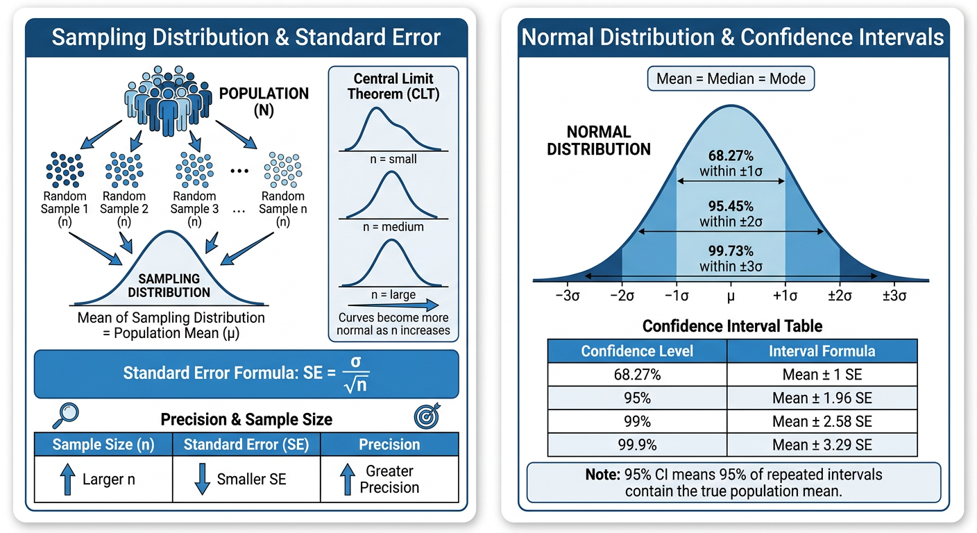
- Sampling Distribution - how sample statistics form their own probability distribution, with the mean equal to the population mean (μ)
- Normal Distribution - the bell curve with the Empirical Rule bands (68.27% / 95.45% / 99.73%)
- Standard Error - the formula SE = σ/√n and the inverse relationship between sample size and precision
- Confidence Intervals - the full table of limits (68.27%, 95%, 99%, 99.9%) with the correct Z multipliers (1, 1.96, 2.58, 3.29), plus the correct interpretation of what a 95% CI actually means
Create a order wise normal distribution ,sampling distribution and standard error and and confidence intervals study guide summarizing hypothesis testing using these concepts
What format do you want the study guide in? · What is the target audience level?
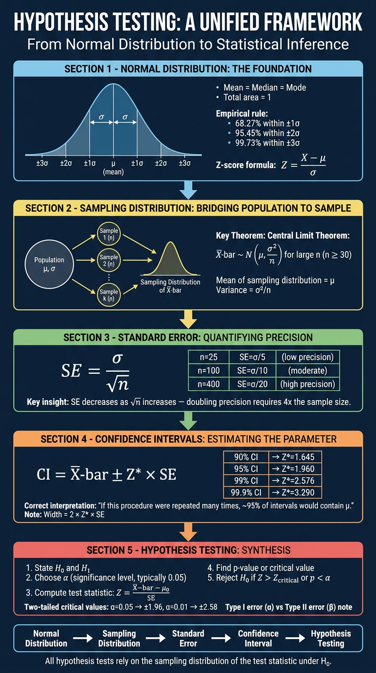
Advanced postgraduate-level statistics study guide poster, tall vertical layout, dark navy blue background with white and light blue text, titled "Hypothesis Testing: A Unified Framework" at the top in large bold white text with subtitle "From Normal Distribution to Statistical Inference". Organized into 5 numbered sequential sections with arrows connecting them top to bottom: SECTION 1 - "Normal Distribution: The Foundation" Bell curve diagram showing symmetrical distribution, labeled: μ (mean), σ (standard deviation). Key properties listed: Mean = Median = Mode, Total area = 1, Empirical rule: 68.27% within ±1σ, 95.45% within ±2σ, 99.73% within ±3σ. Z-score formula: Z = (X - μ) / σ. Light blue section header. SECTION 2 - "Sampling Distribution: Bridging Population to Sample" Diagram showing population → multiple samples of size n → sampling distribution of X-bar. Key theorem: Central Limit Theorem: X-bar ~ N(μ, σ²/n) for large n (n ≥ 30). Mean of sampling distribution = μ. Variance = σ²/n. Yellow section header. SECTION 3 - "Standard Error: Quantifying Precision" Formula prominently displayed: SE = σ / √n. Three-row table: n=25 SE=σ/5 (low precision), n=100 SE=σ/10 (moderate), n=400 SE=σ/20 (high precision). Key insight: SE decreases as √n increases — doubling precision requires 4x the sample size. Green section header. SECTION 4 - "Confidence Intervals: Estimating the Parameter" Formula: CI = X-bar ± Z* × SE. Table with four rows: 90% CI → Z*=1.645, 95% CI → Z*=1.960, 99% CI → Z*=2.576, 99.9% CI → Z*=3.290. Correct interpretation: "If this procedure were repeated many times, ~95% of intervals would contain μ." Note: Width = 2 × Z* × SE. Orange section header. SECTION 5 - "Hypothesis Testing: Synthesis" Step-by-step numbered process: 1. State H₀ and H₁, 2. Choose α (significance level, typically 0.05), 3. Compute test statistic: Z = (X-bar - μ₀) / SE, 4. Find p-value or critical value, 5. Reject H₀ if Z > Z_critical or p < α. Two-tailed critical values: α=0.05 → ±1.96, α=0.01 → ±2.58. Type I error (α) vs Type II error (β) note. Red section header. At the bottom: a horizontal flow diagram showing: Normal Distribution → Sampling Distribution → Standard Error → Confidence Interval → Hypothesis Testing with arrows. Footer text: "All hypothesis tests rely on the sampling distribution of the test statistic under H₀." Clean academic design, well-spaced sections.
-
Normal Distribution - establishes the foundational shape of data and the Z-score formula (Z = (X - μ) / σ). Every parametric test assumes the population (or the sampling distribution) is approximately normal.
-
Sampling Distribution - explains what happens when you repeatedly draw samples. By the Central Limit Theorem, the distribution of sample means X-bar approaches N(μ, σ²/n) regardless of the original population shape, provided n ≥ 30. This is why hypothesis tests work.
-
Standard Error (SE = σ/√n) - quantifies how much sample means vary from the true μ. It is the "spread" of the sampling distribution. Critically, precision scales with √n, not n, so quadrupling sample size only halves the SE.
-
Confidence Intervals (X-bar ± Z × SE)* - use SE to place bounds on where μ likely falls. The multiplier Z* (1.96 for 95%, 2.576 for 99%) comes directly from the normal distribution's cumulative areas.
-
Hypothesis Testing - synthesizes everything. The test statistic Z = (X-bar - μ₀) / SE asks: "How many standard errors is my sample mean from the null hypothesis value?" If it falls in the rejection region (beyond ±1.96 for α = 0.05), you reject H₀. The p-value is simply the area in the tail(s) of the standard normal beyond your computed Z.