
acedemic use of this app for community medicine
Reading File
This is a broad question about the academic use of this app (Orris) for community medicine. Let me clarify what you're looking for before diving in.
Asking for Preferences
What kind of academic use in community medicine are you asking about?
Finding Sources
Finding Sources
Finding Sources
Finding Sources
Finding Sources
Finding Sources
I now have a clear picture of the library and the available community medicine content. Here's a thorough guide to using Orris academically for community medicine:
Using Orris as an Academic Learning Tool for Community Medicine
What's Available in the Library
The app has access to Park's Textbook of Preventive and Social Medicine - the definitive reference for community medicine in medical education. The library also contains supporting textbooks across 30+ specialities that overlap with community medicine topics.
How to Use This App Effectively
1. Ask Conceptual Questions Directly
You can ask about any community medicine topic and get answers sourced from Park's and other authoritative textbooks. For example:
- "What is the WHO definition of health?"
- "Explain the epidemiological triad"
- "What are the levels of prevention with examples?"
- "Define herd immunity and its threshold"
The app retrieves exact passages from textbooks, so you get accurate, citable answers - not paraphrased summaries.
2. Topics Covered in Park's (Available in This App)
The textbook covers the full community medicine curriculum:
| Domain | Example Topics |
|---|---|
| Concepts of Health & Disease | WHO definition, dimensions of health, biomedical/ecological/psychosocial/holistic concepts |
| History of Medicine | Primitive medicine, germ theory, Primary Health Care, SDGs, Health for All |
| Epidemiology | Descriptive/analytical epidemiology, study designs, measures of disease frequency |
| Biostatistics | Data types, normal distribution, tests of significance, sampling |
| Environment & Health | Water, air, food hygiene; sanitation; vector control |
| Nutrition | Nutritional disorders, PEM, vitamin deficiencies, national nutrition programs |
| Communicable Diseases | Respiratory, enteric, vector-borne, sexually transmitted diseases |
| Non-communicable Diseases | CVD, cancer, diabetes, mental health |
| Health Care & Planning | Primary health care, health systems, national health policy |
| Demography | Census, birth/death rates, population dynamics |
| National Health Programs | RNTCP, NVBDCP, NRHM, immunization schedules |
| Occupational & Environmental Health | Occupational diseases, industrial hazards |
| Family Medicine | Family health, MCH, school health |
| Social Medicine | Poverty, social determinants, Millennium/Sustainable Development Goals |
3. Cross-Specialty Learning
Community medicine overlaps with many other specialities. This app has textbooks in all relevant areas:
- Microbiology - for communicable disease agents
- Pharmacology - for vaccines and drug programs
- Pediatrics - for immunization and child health programs
- Obstetrics & Gynecology - for maternal health programs
- Psychiatry - for mental health in the community
- Internal Medicine - for NCD management at population level
- Genetics / Epidemiology - for disease burden studies
You can ask questions that span these areas (e.g., "How is TB managed under RNTCP?") and get combined answers from multiple sources.
4. Evidence-Based Study
Beyond textbooks, this app can search PubMed for recent studies. This is useful when you need:
- Latest WHO/government guidelines
- Recent meta-analyses on public health interventions
- Current data on disease burden
Example: "What is the latest evidence on oral rehydration therapy in childhood diarrhea?"
5. Practical Use Cases for Students
| Academic Task | How to Use This App |
|---|---|
| Exam revision | Ask direct questions: "Define sensitivity and specificity" |
| MCQ clarification | Paste an MCQ you're unsure about and ask for an explanation |
| Case discussions | Describe a community-level scenario (e.g., a disease outbreak) and ask for analysis |
| Essay/structured answers | Ask "Outline the control measures for malaria" for structured content |
| Comparing concepts | "Difference between incidence and prevalence" |
| Health program details | "What are the components of the Universal Immunization Programme?" |
| Biostatistics help | "When do I use chi-square vs Fisher's exact test?" |
| Journal reading | Ask for a summary or explanation of any PubMed paper |
6. Tips for Best Results
- Be specific - Instead of "tell me about epidemiology", ask "What are the types of epidemiological studies and their hierarchy of evidence?"
- Ask for definitions - Great for one-liners needed in exams (e.g., "Define attack rate")
- Ask for comparisons - "Compare case-control vs cohort studies"
- Ask for diagrams/tables - The app can retrieve textbook images and diagrams where available
- Ask follow-up questions - The app remembers context within a conversation, so you can dig deeper after a first answer
7. What This App Does NOT Replace
- Clinical field postings and community visits
- Practical skills (surveys, data collection, field epidemiology)
- Your college's exam-specific syllabus weightage
- Real-time government program updates (though web search covers these)
In short, treat this app like having Park's Textbook open alongside a medical search engine, a PubMed terminal, and a tutor who can explain and connect concepts - all at once. It works best when you ask focused, topic-specific questions rather than broad requests.
Want to try it out with a specific community medicine topic right now?
Biostatistics Data types, normal distribution, tests of significance, sampling explain this topic in comprehensive way with example
Finding Sources
Finding Sources
Finding Sources
Finding Sources
Finding Sources
Finding Sources
Now let me read the actual Park's content on these topics:
Reading File
Reading File
Reading File
Reading File
Reading File
Reading File
Reading File
I now have all the core content from Park's. Let me also fetch the normal curve image and get the tests of significance content:
Loading Image
Reading File
Reading File
I now have all the content needed from Park's Textbook. Let me compile the comprehensive answer:
Biostatistics - Comprehensive Guide for Community Medicine
Source: Park's Textbook of Preventive and Social Medicine, pp. 944-960
PART 1: DATA TYPES
What is Data?
Data = discrete observations that carry little meaning alone. They must be transformed into information (by summarizing/adjusting) and then into intelligence (by integrating with experience) to guide decision-making in public health.
Types of Data
Data in biostatistics is broadly classified as:
| Type | Sub-type | Definition | Example |
|---|---|---|---|
| Qualitative (Categorical) | Nominal | Categories with no natural order | Blood group (A, B, AB, O); sex (M/F); religion |
| Ordinal | Categories with a natural rank order | Disease severity (mild, moderate, severe); socioeconomic status | |
| Quantitative (Numerical) | Discrete | Counts; only whole numbers possible | Number of children in a family; number of malaria cases |
| Continuous | Any value within a range (measurable) | Height, weight, hemoglobin, blood pressure, temperature |
Key Distinctions with Examples
Nominal data - you can only count frequencies. You cannot say blood group B is "more" than blood group A.
Ordinal data - you can rank, but the gap between ranks is unequal. The difference between "mild" and "moderate" is not necessarily the same as between "moderate" and "severe."
Discrete data - Example: A family has 2 or 3 children, never 2.5.
Continuous data - Example: Hemoglobin can be 11.4 g/dL, 11.41 g/dL, etc. Limited only by measuring precision.
Rule for choosing statistics: The type of data determines what statistical test is appropriate. Never apply a mean to nominal data (you can't calculate the average blood group).
PART 2: NORMAL DISTRIBUTION
The Concept
If you measure hemoglobin (or height, weight, blood pressure) in a very large number of people and plot it as a frequency distribution with narrow class intervals, you get a smooth, symmetrical, bell-shaped curve - the normal curve (also called Gaussian distribution).
The shape depends on the mean (x̄) and standard deviation (σ), meaning there can be an infinite number of normal curves depending on the population studied.
The Bell Curve - The 68-95-99.7 Rule
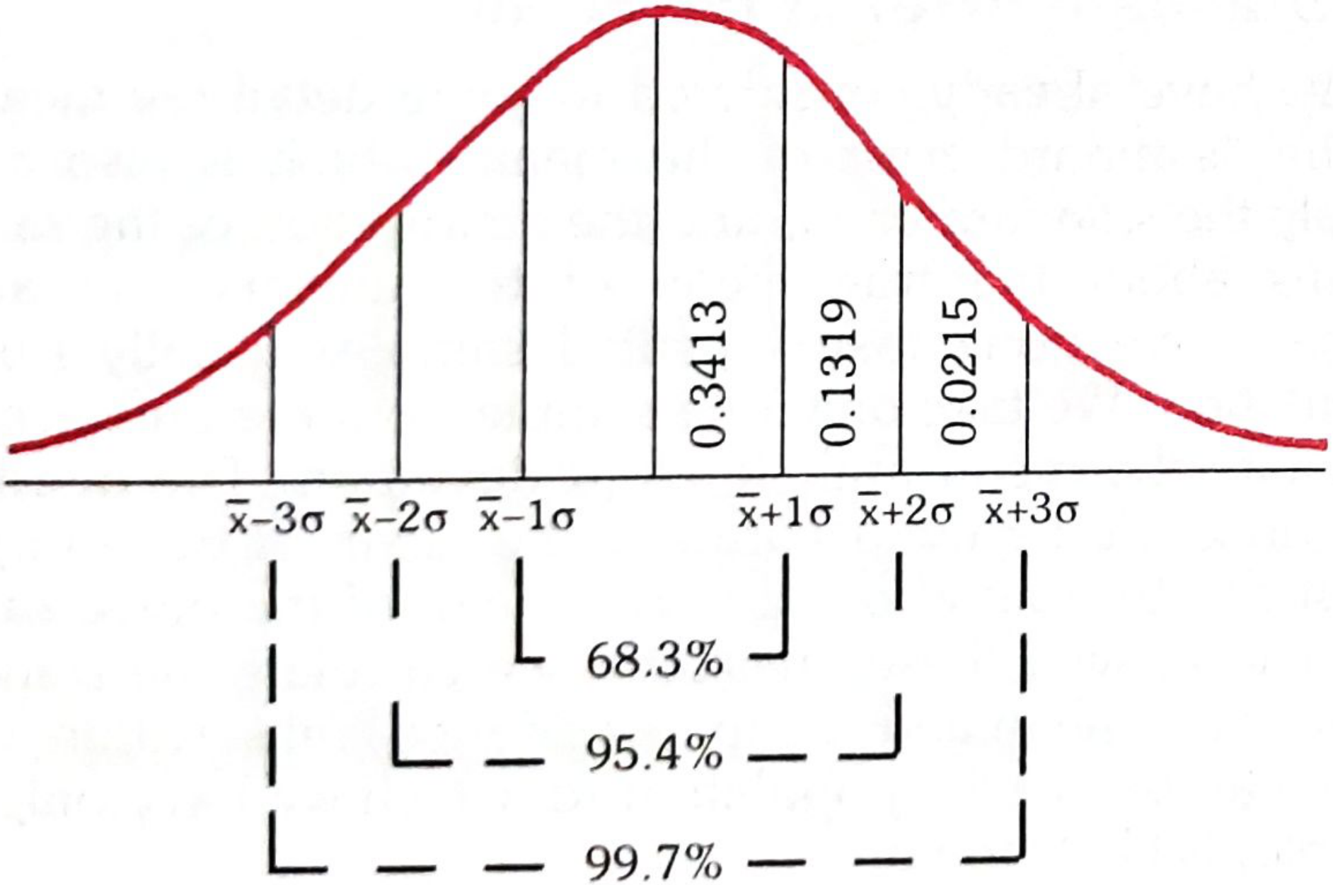
Fig. 15 from Park's Textbook - Normal Curve
| Range | % of values included | Interpretation |
|---|---|---|
| x̄ ± 1σ | 68.3% | ~2 in 3 values fall here |
| x̄ ± 2σ | 95.4% | Most values; used as clinical normal range |
| x̄ ± 3σ | 99.7% | Almost all values |
These limits on either side of the mean are called confidence limits.
At x̄ ± 2σ (95% confidence limits): the probability of a reading falling outside this range is 1 in 20, i.e., P = 0.05.
Properties of the Normal Curve
- Perfectly symmetrical (bell-shaped)
- Mean = Median = Mode (all coincide at the center)
- The tails extend to infinity but never touch the x-axis
- Total area under the curve = 1 (or 100%)
Standard Normal Curve (Z-score)
There is only one standardized normal curve: mean = 0, standard deviation = 1.
Z-score formula:
Z = (x - x̄) / σ
Z tells you how many standard deviations a value is away from the mean.
Example from Park's:
Pulse rate of healthy males: mean = 72, SD = 2.
What is the probability of finding a male with pulse ≥ 80?
Z = (80 - 72) / 2 = 4
From the standard normal table, area at Z = 4 is 0.49997.
Area beyond 4SD = 0.5 - 0.49997 = 0.00003
→ Only 3 in 100,000 individuals would have a pulse of 80 or above. This is extremely rare.
PART 3: SAMPLING
Why Sample?
When studying a large population, it is easier and more economical to study a sample (a subset) rather than the entire population (universe). The key requirement: the sample must be representative of the whole population.
Sampling Frame
Before sampling, you need a sampling frame - a complete listing of all members of the universe from which the sample will be drawn. The accuracy and completeness of this frame determines the quality of the sample.
Example: If you want to study blood pressure in adults of Pune city, your sampling frame = the electoral rolls or census list of all adults in Pune.
Types of Sampling Methods (from Park's)
1. Simple Random Sampling
Every unit has an equal chance of being selected.
- Method: Assign a number to every unit in the sampling frame, then use a table of random numbers to select the required sample.
- Example: From 500 patients in a hospital registry, you want 50. Number them 001-500, use random number tables to pick 50 numbers.
- Advantage: Eliminates selection bias.
- Disadvantage: Requires a complete sampling frame; difficult for large dispersed populations.
2. Systematic Sampling
Select every k-th unit from the list, where k = population size / sample size.
- Example: You need 100 from 1000 patients. k = 1000/100 = 10. Randomly pick a starting number (say 7), then select 7, 17, 27, 37... and so on.
- Advantage: Simple and quick.
- Disadvantage: Risk of bias if the list has a periodic pattern.
3. Stratified Random Sampling
Divide the population into strata (subgroups based on age, sex, religion, etc.), then take a random sample from each stratum.
- Example: To study malnutrition in children, divide by age group (0-1, 1-3, 3-5 years) and sample separately from each group.
- Advantage: Ensures all subgroups are represented; increases precision.
4. Cluster Sampling
Divide the population into clusters (usually geographic), randomly select some clusters, and study all individuals within the selected clusters.
- Example: To survey vaccine coverage in a district, randomly select 10 villages (clusters) and interview every child in those villages.
- Advantage: Practical and economical for large field surveys.
- Disadvantage: Less precise than simple random sampling; clusters may be homogeneous (clustering effect).
5. Multi-stage Sampling
Sampling is done in successive stages - first select large units (e.g., states), then smaller units within them (districts), then smaller still (villages).
- Used in: National Sample Surveys, NFHS (National Family Health Survey).
- Example: State → District → Block → Village → Household
Summary Table
| Method | Best for | Key feature |
|---|---|---|
| Simple random | Small, defined populations | Random number table |
| Systematic | Ordered lists | Every k-th unit |
| Stratified | Heterogeneous populations | Proportional representation |
| Cluster | Large field surveys | Geographic units |
| Multi-stage | National surveys | Stages of selection |
PART 4: TESTS OF SIGNIFICANCE
The Core Concept
A test of significance answers: Is the observed difference between two groups a real difference, or could it have occurred by chance?
The tool used is the standard error (SE) - the standard deviation of the sampling distribution of means. It measures how reliable a sample estimate is.
Formula:
SE of mean = s / √n
Where s = sample standard deviation, n = sample size.
The larger the sample, the smaller the SE - i.e., more precise estimates.
Understanding P-value
- P < 0.05 (1 in 20): The difference is considered significant - unlikely due to chance
- P < 0.01 (1 in 100): The difference is more significant
- P > 0.05: The difference is not significant - could be due to chance
(a) Standard Error of the Mean
Example from Park's:
Random sample of 25 males (age 20-24); mean temperature = 98.14°F, SD = 0.6.
SE = 0.6 / √25 = 0.12
95% confidence limits = 98.14 ± (2 × 0.12) = 97.90°F to 98.38°F
Interpretation: There is only a 1 in 20 chance (P = 0.05) that the true population mean lies outside this range.
(b) Standard Error of Proportion
Used when data is in proportions (e.g., percentage of males, percentage immune).
Formula:
SE of proportion = √(pq/n)
Example from Park's:
In a village, males = 52%. A sample of 100 people shows only 40% males. Is this significant?
SE = √(52 × 48 / 100) = 5.0
95% limits = 52 ± 2(5) = 42 to 62%
The observed 40% falls outside this range.
Relative deviate = (52 - 40) / 5 = 2.4
Since 2.4 > 2.0, the difference is statistically significant - this sample is not representative of the village population.
(c) Standard Error of Difference Between Two Means
Used to compare means of two independent groups (e.g., control vs. experimental).
Example from Park's (drug effect on kidney weight in mice):
| Group | n | Mean (mg) | SD |
|---|---|---|---|
| Control | 12 | 318 | 10.2 |
| Drug-treated | 12 | 326 | 9.8 |
If the SE of difference is calculated and the observed difference (326 - 318 = 8 mg) divided by SE exceeds 2, the difference is significant at P < 0.05.
(d) Standard Error of Difference Between Two Proportions
Used when comparing proportions from two different populations.
Formula:
SE diff = √[ p₁q₁/n₁ + p₂q₂/n₂ ]
If (p₁ - p₂) / SE diff > 2 → significant difference
Common Tests and When to Use Them
| Test | Data type | Use when |
|---|---|---|
| Z-test / SE test | Continuous (large n) | Comparing means, n > 30 |
| t-test | Continuous (small n) | Comparing means, n < 30 |
| Chi-square (χ²) | Categorical / proportions | Comparing frequencies in 2×2 or larger tables |
| Fisher's exact test | Categorical | Chi-square when expected cell count < 5 |
| ANOVA | Continuous | Comparing means of 3 or more groups |
| Correlation (r) | Continuous (both variables) | Association between two continuous variables |
Quick Memory Map
DATA TYPES
├── Qualitative → Nominal (no order) / Ordinal (ranked)
└── Quantitative → Discrete (count) / Continuous (measured)

NORMAL DISTRIBUTION
├── Bell-shaped, symmetrical
├── Mean = Median = Mode
└── 68% → 95% → 99.7% rule (1σ / 2σ / 3σ)

SAMPLING
├── Random → equal chance for all
├── Systematic → every k-th unit
├── Stratified → subgroup representation
├── Cluster → geographic groups
└── Multi-stage → stages of selection

TESTS OF SIGNIFICANCE
├── SE of mean → is our sample mean reliable?
├── SE of proportion → is our % estimate reliable?
├── SE of difference (means) → are 2 groups truly different?
└── P < 0.05 = significant; P > 0.05 = not significant
All content sourced from Park's Textbook of Preventive and Social Medicine, pp. 944-960, the standard reference for community medicine biostatistics.
Explain common statistical tests (t-test, chi-square) with clinical examples
Searching the medical library for detailed content on t-test and chi-square from Park's and other textbooks.
Finding Sources
Finding Sources
Reading File
Reading File
Reading File
Reading File
Reading File
Reading File
Your credits are exhausted. Your daily credits reset tomorrow, or you can purchase a top-up for more.
Occupational diseases, industrial hazards exlain
Your credits are exhausted. Your daily credits reset tomorrow, or you can purchase a top-up for more.
This is a shared conversation. Sign in to Orris to start your own chat.