
Biostatisticsh * Normal distribution * Hypothesis testing * p value * Chi-square test * t-test * Errors in hypothesis testing * Measures of central tendency. * Chi-square test.
Reading File
Now let me search the medical library for biostatistics content across all these topics in parallel.
Finding Sources
Finding Sources
Excellent finds. Now let me read the most relevant sections in parallel - Park's Textbook (preventive medicine, most relevant for biostatistics), Henry's Clinical Diagnosis (chi-square, t-test), and Barash/Goldman for hypothesis testing.
Reading File
Reading File
Reading File
Excellent content. Now let me read the remaining sections - chi-square and t-test from Henry's, and the measures of central tendency + p-value + errors from Park's.
Reading File
Reading File
Now let me read the p-value, errors, measures of central tendency, and chi-square sections from Park's - and more chi-square from Henry's.
Reading File
Reading File
Now let me get the measures of central tendency and errors in hypothesis testing sections from Park's.
Reading File
Now let me fetch the normal distribution image and get earlier content for measures of central tendency (mean/mode) and errors in hypothesis testing.
Loading Image
Reading File
Reading File
Now I have the normal distribution image. Let me get measures of central tendency (mean/mode) from Park's which will be earlier in the file, and the errors + chi-square sections.
Reading File
Reading File
Now let me read the chi-square result and errors section from Park's.
Reading File
I need the errors in hypothesis testing section and the mode section. Let me get the mode from Park's and the errors section.
Reading File
Reading File
I need the Type I and Type II errors section. Let me search specifically for that.
Finding Sources
Reading File
Reading File
I now have comprehensive content from the textbooks covering all topics. Let me also get the p-value section from Goldman-Cecil and the Sabiston errors section for depth.
Reading File
I now have thorough content from multiple authoritative medical textbooks. Let me compile the comprehensive answer.
Biostatistics: A Complete Overview
Sources: Park's Textbook of Preventive and Social Medicine; Henry's Clinical Diagnosis and Management by Laboratory Methods; Goldman-Cecil Medicine; Barash Clinical Anesthesia; Miller's Review of Orthopaedics
1. Measures of Central Tendency
The "average" gives a mental picture of the central value in a distribution. There are three commonly used measures:
(a) The Mean (Arithmetic Mean)
Individual observations are summed and divided by the number of observations.
Example: Diastolic BP of 10 individuals = 83, 75, 81, 79, 71, 95, 75, 77, 84, 90. Total = 810. Mean = 810/10 = 81.0
Advantages: Easy to calculate and understand.
Disadvantages: Unduly influenced by extreme (outlier) values.
(b) The Median
Data is arranged in ascending/descending order; the middle value is the median. If n is even, take the average of the two middle values.
Example: BP of 9 individuals arranged: 71, 75, 75, 77, 79, 81, 83, 84, 95 → Median = 79
Advantage: Not affected by extreme values - more representative when outliers are present (e.g., incomes).
(c) The Mode
The most frequently occurring value in a distribution.
Example: In the series 85, 75, 81, 79, 71, 95, 75, 77, 75, 90... the value 75 appears most often → Mode = 75
Advantage: Not affected by extreme items. Disadvantage: Often not clearly defined; seldom used in biological statistics.
Comparison: In a perfectly normal distribution, Mean = Median = Mode. When extreme values are present, Median > Mean is often more representative.
- Park's Textbook of Preventive and Social Medicine, pp. 951-952
2. Normal Distribution
The normal distribution (also called the Gaussian or bell curve) is the cornerstone of statistical theory. When data from a large population (e.g., haemoglobin values) is plotted with narrow class intervals, a smooth, symmetrical bell-shaped curve emerges.
Mathematical Formula
$$P(x) = \frac{1}{\sigma\sqrt{2\pi}} e^{-\frac{(x-\bar{x})^2}{2\sigma^2}}$$
Key Properties of the Normal Curve
- Perfectly symmetrical about the mean
- Mean = Median = Mode (all coincide at the centre)
- The curve extends to ±∞ but the tails approach (never touch) the x-axis
- The total area under the curve = 1 (100%)
The 68-95-99.7 Rule (Critical for Exams)
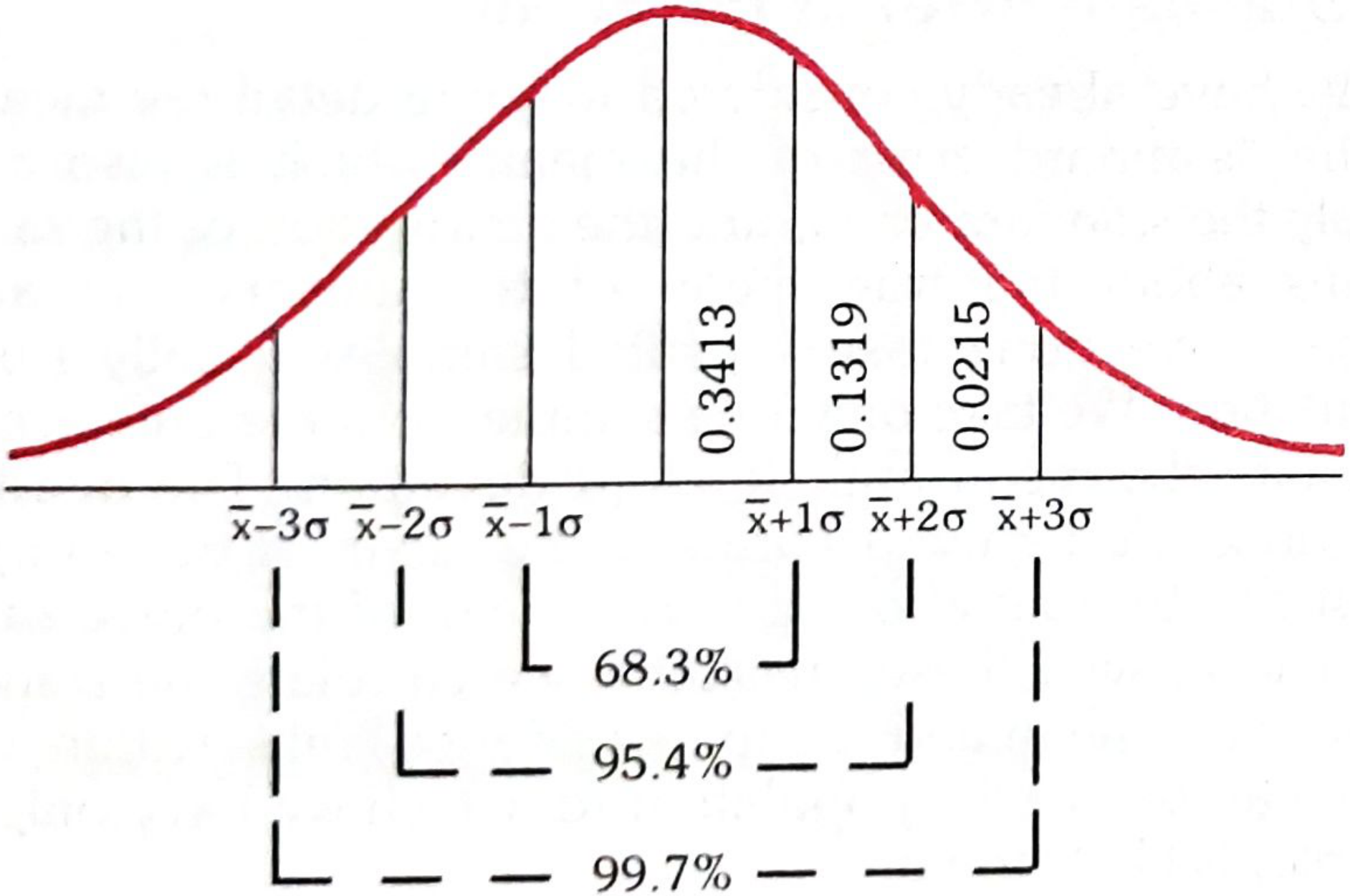
| Range | % of Values |
|---|---|
| x̄ ± 1σ | 68.3% |
| x̄ ± 2σ | 95.4% (~95%) |
| x̄ ± 3σ | 99.7% |
Standard Normal Curve (Z-distribution)
There is only one standardized normal curve with:
- Mean = 0
- SD = 1
The Z-score (standard normal variate) converts any raw value to this scale:
$$Z = \frac{x - \bar{x}}{\sigma}$$
Clinical use: The normal reference range for a laboratory analyte is calculated as mean ± 2 SD, capturing the central 95% of values in a healthy population.
- Park's Textbook of Preventive and Social Medicine, pp. 952-954
- Henry's Clinical Diagnosis and Management by Laboratory Methods, p. 130
3. Hypothesis Testing
Hypothesis testing determines whether an observed difference between groups is real or due to chance.
The Two Hypotheses
- Null Hypothesis (H₀): States there is NO difference between groups (e.g., a drug has no effect).
- Alternative Hypothesis (H₁): States there IS a significant difference.
The Process
- State H₀ and H₁
- Choose the appropriate statistical test
- Calculate the test statistic
- Find the p-value
- Compare to alpha (α) threshold (usually 0.05)
- Reject or fail to reject H₀
"The statistical question for consideration is reduced to two mutually exclusive hypotheses. If the t-statistic has a sufficiently high value, we reject H₀ and accept H₁. This decision is like a trial verdict: 'guilty' vs 'not guilty' - innocence is never established, and similarly H₀ is never proven, only failed to be rejected." - Henry's Clinical Diagnosis
Choosing the Right Test (Goldman-Cecil Table)
| Type of Outcome Variable | Statistical Method |
|---|---|
| Categorical (dichotomous) | 2×2 table, Chi-square |
| Categorical (nominal) | Chi-square |
| Continuous (two groups) | t-test |
| Continuous (>2 groups) | ANOVA |
| Ordinal | Mann-Whitney |
- Goldman-Cecil Medicine, p. 2694-2696
- Barash Clinical Anesthesia, p. 523
4. P-Value
The p-value is the probability that the observed difference (or more extreme) occurred by chance alone, assuming the null hypothesis is true.
| P-value | Interpretation |
|---|---|
| p < 0.05 | Statistically significant (less than 5% chance it's due to chance) |
| p = 0.05 | Just significant (borderline) |
| p > 0.05 | Not significant (difference may be due to chance) |
The conventional threshold is p < 0.05 (5% level). This means we accept a 1 in 20 chance of being wrong when calling a result "significant."
Confidence Limits and P-value
When the 95% confidence interval does NOT include the null value (zero for differences, 1.0 for ratios), p < 0.05.
Example from Barash: In an RCT comparing lidocaine vs bupivacaine, 9/35 vs 1/35 patients had transient neurologic symptoms. Chi-square = 5.72, p = 0.017 → significant difference.
- Park's Textbook of Preventive and Social Medicine, p. 955
5. Errors in Hypothesis Testing
Even with careful testing, two fundamental errors are possible:
Type I Error (Alpha Error, α)
- Incorrectly rejecting the null hypothesis
- Concluding groups ARE different when they actually are NOT
- = "False Positive"
- Acceptable probability: ≤ 0.05 (5%)
- Represents the p-value threshold
"A Type I error occurs when a null hypothesis is rejected although it is true. To eliminate any possibility would necessitate an infinite number of subjects, so by convention a 5% chance is accepted." - Goldman-Cecil Medicine
Type II Error (Beta Error, β)
- Incorrectly failing to reject the null hypothesis
- Concluding groups are NOT different when they actually ARE
- = "False Negative"
- Acceptable probability: up to 20%
- Related to statistical power (Power = 1 − β)
| H₀ True (no real difference) | H₀ False (real difference exists) | |
|---|---|---|
| Reject H₀ | ❌ Type I error (α) | ✅ Correct (True Positive) |
| Fail to Reject H₀ | ✅ Correct (True Negative) | ❌ Type II error (β) |
Power
Power = 1 − β = probability of correctly detecting a true difference. A well-designed study aims for power ≥ 80%. Power increases with larger sample sizes.
- Henry's Clinical Diagnosis, p. 130
- Goldman-Cecil Medicine, p. 2698
- Miller's Review of Orthopaedics, p. 110-120
6. The t-Test (Student's t-Test)
The t-test is the most common method for comparing a continuous variable between two groups.
History
Devised by William Gosset under the pseudonym "Student" while working for the Guinness brewery - he wanted to keep his work for optimizing productivity unrecognized by competitors.
Formula
$$t = \frac{\bar{x}_1 - \bar{x}_2}{SD_c\sqrt{\frac{1}{n_1} + \frac{1}{n_2}}}$$
Where:
- x̄₁, x̄₂ = mean values of groups 1 and 2
- n₁, n₂ = number of values in each group
- SDc = combined standard deviation of both groups
Types of t-Tests
| Type | Use |
|---|---|
| Unpaired (independent) | Two separate, unrelated groups (e.g., males vs females) |
| Paired | Same subjects measured twice (e.g., before/after treatment) |
Assumptions for Validity
- Data must be approximately normally distributed
- Approximately equal numbers in each group
- Variances of the groups should be equivalent
- Observations must be independent of each other (no patient appears twice)
Interpretation
- Calculate t-statistic
- Find degrees of freedom (df = n₁ + n₂ − 2)
- Look up p-value
- If p < 0.05 → reject H₀ → means are significantly different
Example: Hemoglobin in males (mean 15.1, SD 0.96, n=36) vs females (mean 13.2, SD 0.80, n=49). t = 9.898, p < 0.001 → significant difference.
- Henry's Clinical Diagnosis, pp. 154-155
7. Chi-Square Test (χ²)
The chi-square test is used for categorical (nominal) data arranged in a contingency table. It tests whether an observed distribution differs from what would be expected if there were no association.
When to Use
- Comparing proportions between two or more groups
- Data is in frequency counts (not means)
- Ideal for 2×2 contingency tables (can extend to larger tables)
Formula
$$\chi^2 = \sum \frac{(O - E)^2}{E}$$
Where:
- O = Observed frequency in each cell
- E = Expected frequency (calculated from marginal totals)
Step-by-Step Method (Park's Vaccine Example)
Data: Whooping cough vaccine trial: Vaccine A (22 attacked/90) vs Vaccine B (14 attacked/86).
Step 1 - State the Null Hypothesis: No difference between the two vaccines.
Step 2 - Calculate Expected Values:
Overall attack rate = 36/176 = 0.204
- Expected attacks, Vaccine A = 90 × 0.204 = 18.36
- Expected attacks, Vaccine B = 86 × 0.204 = 17.54
Step 3 - Apply the χ² formula:
$$\chi^2 = \frac{(22-18.36)^2}{18.36} + \frac{(68-71.55)^2}{71.55} + \frac{(14-17.54)^2}{17.54} + \frac{(72-68.37)^2}{68.37}$$
$$= 0.72 + 0.17 + 0.71 + 0.19 = \mathbf{1.79}$$
Step 4 - Degrees of Freedom:
$$df = (r-1)(c-1) = (2-1)(2-1) = 1$$
Step 5 - Interpret using table:
Critical χ² value at df=1, p=0.05 → 3.84
Since 1.79 < 3.84 → p > 0.05 → Fail to reject H₀ → No significant difference between vaccines.
Assumptions (Critical!)
- Each cell must have an expected value ≥ 5 (some sources say ≥ 2)
- When cell sizes are small (< 5), use Fisher's Exact Test instead
- Total sample size should be reasonably large
- Data must be in counts, not percentages
Chi-square for 2×2 Tables - Quick Reference
| Disease + | Disease - | Total | |
|---|---|---|---|
| Exposed | a | b | a+b |
| Unexposed | c | d | c+d |
| Total | a+c | b+d | n |
Expected value for cell 'a' = (a+b)(a+c)/n
- Park's Textbook of Preventive and Social Medicine, pp. 956-957
- Henry's Clinical Diagnosis, pp. 154-155
- Barash Clinical Anesthesia, p. 523
Quick Comparison Summary
| Feature | t-Test | Chi-Square |
|---|---|---|
| Data type | Continuous (means) | Categorical (counts) |
| Groups | 2 groups | 2+ groups |
| Assumption | Normal distribution | Expected freq ≥ 5 |
| Tests | Difference of means | Association between variables |
| When cell sizes small | Use Welch's t-test | Use Fisher's Exact Test |
Exam Mnemonics
- "ALPHA = Alarm" (Type I) - You falsely set off the alarm (false positive)
- "BETA = Blind" (Type II) - You're blind to the real difference (false negative)
- Z-score rule: 1σ = 68%, 2σ = 95%, 3σ = 99.7%
- Chi-square uses O and E → "Observed vs Expected"
- p < 0.05 = statistically significant (less than 5% probability of chance)
Make a pdf
Reading File
Running Command
mkdir -p /tmp/workspace/biostatistics-pdf && ls /tmp/workspace/
Writing File
~/biostatistics-pdf/generate_pdf.py
from reportlab.lib.pagesizes import A4
from reportlab.lib.styles import getSampleStyleSheet, ParagraphStyle
from reportlab.lib.units import cm
from reportlab.lib import colors
from reportlab.platypus import (
SimpleDocTemplate, Paragraph, Spacer, Table, TableStyle,
HRFlowable, PageBreak, KeepTogether
)
from reportlab.lib.enums import TA_CENTER, TA_LEFT, TA_JUSTIFY
from reportlab.platypus import Image
import urllib.request
import os
OUTPUT = "/tmp/workspace/biostatistics-pdf/Biostatistics_Notes.pdf"
# ---------- Styles ----------
styles = getSampleStyleSheet()
TEAL = colors.HexColor("#0D7377")
DARK_TEAL = colors.HexColor("#14A085")
LIGHT_BG = colors.HexColor("#F0F8F7")
ACCENT = colors.HexColor("#E8F5F4")
YELLOW = colors.HexColor("#FFF8E1")
DARK_GRAY = colors.HexColor("#2C3E50")
MID_GRAY = colors.HexColor("#5D6D7E")
TABLE_HDR = colors.HexColor("#0D7377")
TABLE_ALT = colors.HexColor("#EAF6F6")
RED_BOX = colors.HexColor("#FDEDEC")
RED_BDR = colors.HexColor("#E74C3C")
GREEN_BOX = colors.HexColor("#EAFAF1")
GREEN_BDR = colors.HexColor("#27AE60")
cover_title = ParagraphStyle("cover_title",
fontSize=34, fontName="Helvetica-Bold",
textColor=colors.white, alignment=TA_CENTER,
spaceAfter=10, leading=42)
cover_sub = ParagraphStyle("cover_sub",
fontSize=16, fontName="Helvetica",
textColor=colors.HexColor("#D5F5E3"), alignment=TA_CENTER,
spaceAfter=6)
cover_src = ParagraphStyle("cover_src",
fontSize=10, fontName="Helvetica-Oblique",
textColor=colors.HexColor("#A9DFBF"), alignment=TA_CENTER)
h1 = ParagraphStyle("h1",
fontSize=20, fontName="Helvetica-Bold",
textColor=colors.white, alignment=TA_LEFT,
spaceBefore=4, spaceAfter=4, leading=26,
backColor=TEAL,
borderPad=(6, 10, 6, 10))
h2 = ParagraphStyle("h2",
fontSize=14, fontName="Helvetica-Bold",
textColor=TEAL, spaceBefore=14, spaceAfter=4,
borderPad=2, leading=18)
h3 = ParagraphStyle("h3",
fontSize=11, fontName="Helvetica-Bold",
textColor=DARK_GRAY, spaceBefore=10, spaceAfter=3,
leading=15)
body = ParagraphStyle("body",
fontSize=10, fontName="Helvetica",
textColor=DARK_GRAY, spaceAfter=6,
leading=15, alignment=TA_JUSTIFY)
bullet = ParagraphStyle("bullet",
fontSize=10, fontName="Helvetica",
textColor=DARK_GRAY, leftIndent=16, spaceAfter=4,
leading=14, bulletIndent=6)
formula = ParagraphStyle("formula",
fontSize=11, fontName="Courier-Bold",
textColor=TEAL, backColor=ACCENT,
spaceAfter=6, spaceBefore=4,
leftIndent=20, rightIndent=20,
borderPad=8, leading=16)
example_style = ParagraphStyle("example",
fontSize=9.5, fontName="Helvetica-Oblique",
textColor=MID_GRAY, leftIndent=20, spaceAfter=4,
leading=13, backColor=YELLOW,
borderPad=6)
note_style = ParagraphStyle("note",
fontSize=9.5, fontName="Helvetica",
textColor=colors.HexColor("#1A5276"),
backColor=colors.HexColor("#EBF5FB"),
spaceAfter=6, spaceBefore=4,
leftIndent=10, rightIndent=10,
borderPad=6, leading=13)
mnemonic = ParagraphStyle("mnemonic",
fontSize=10, fontName="Helvetica-Bold",
textColor=colors.HexColor("#6C3483"),
backColor=colors.HexColor("#F5EEF8"),
spaceAfter=4, spaceBefore=4,
leftIndent=10, rightIndent=10,
borderPad=6, leading=14)
sources_style = ParagraphStyle("sources",
fontSize=8, fontName="Helvetica-Oblique",
textColor=MID_GRAY, spaceAfter=3, leading=11)
# ---------- Helper: section header ----------
def section_header(num, title):
return [
Spacer(1, 10),
Table([[Paragraph(f"{num}. {title}", h1)]],
colWidths=[17*cm],
style=TableStyle([
("BACKGROUND", (0,0), (-1,-1), TEAL),
("ROUNDEDCORNERS", [6]),
("TOPPADDING", (0,0), (-1,-1), 8),
("BOTTOMPADDING", (0,0), (-1,-1), 8),
("LEFTPADDING", (0,0), (-1,-1), 14),
])),
Spacer(1, 6),
]
def sub_header(text):
return Paragraph(text, h2)
def sub_sub(text):
return Paragraph(text, h3)
def para(text):
return Paragraph(text, body)
def bul(text):
return Paragraph(f"\u2022 {text}", bullet)
def form(text):
return Paragraph(text, formula)
def ex(text):
return Paragraph(f"\u25b6 {text}", example_style)
def note(text):
return Paragraph(f"\u2139 {text}", note_style)
def mnemo(text):
return Paragraph(f"\U0001f9e0 {text}", mnemonic)
def hr():
return HRFlowable(width="100%", thickness=1, color=colors.HexColor("#BDC3C7"), spaceAfter=6, spaceBefore=6)
# ---------- Generic table builder ----------
def build_table(headers, rows, col_widths=None):
if col_widths is None:
col_widths = [17*cm/len(headers)] * len(headers)
hdr_row = [Paragraph(f"<b>{h}</b>", ParagraphStyle("th",
fontSize=9.5, fontName="Helvetica-Bold",
textColor=colors.white, alignment=TA_CENTER, leading=12)) for h in headers]
data = [hdr_row]
for i, row in enumerate(rows):
data.append([Paragraph(str(c), ParagraphStyle("td",
fontSize=9, fontName="Helvetica",
textColor=DARK_GRAY, leading=12)) for c in row])
ts = TableStyle([
("BACKGROUND", (0,0), (-1,0), TABLE_HDR),
("ROWBACKGROUNDS", (0,1), (-1,-1), [colors.white, TABLE_ALT]),
("GRID", (0,0), (-1,-1), 0.5, colors.HexColor("#BDC3C7")),
("TOPPADDING", (0,0), (-1,-1), 5),
("BOTTOMPADDING", (0,0), (-1,-1), 5),
("LEFTPADDING", (0,0), (-1,-1), 7),
("RIGHTPADDING", (0,0), (-1,-1), 7),
("VALIGN", (0,0), (-1,-1), "MIDDLE"),
])
return Table(data, colWidths=col_widths, style=ts, hAlign="LEFT")
# ---------- Download normal curve image ----------
img_path = "/tmp/workspace/biostatistics-pdf/normal_curve.png"
try:
urllib.request.urlretrieve(
"https://cdn.orris.care/cdss_images/c39869747094c8561f90f8f17758c9d8d4517297107f9e433d6f95463ff6982f.png",
img_path)
print("Image downloaded OK")
except Exception as e:
print(f"Image download failed: {e}")
img_path = None
# ---------- Document ----------
doc = SimpleDocTemplate(
OUTPUT, pagesize=A4,
leftMargin=2*cm, rightMargin=2*cm,
topMargin=2*cm, bottomMargin=2*cm,
title="Biostatistics Notes",
author="Orris Medical")
story = []
# ===== COVER PAGE =====
story.append(Spacer(1, 1.5*cm))
cover_tbl = Table(
[[Paragraph("BIOSTATISTICS", cover_title)],
[Paragraph("Complete Study Notes", cover_sub)],
[Paragraph("Normal Distribution • Hypothesis Testing • p-Value\n"
"t-Test • Chi-Square Test • Errors • Central Tendency", cover_sub)],
[Spacer(1, 12)],
[Paragraph("Sources: Park's Textbook of Preventive & Social Medicine | "
"Henry's Clinical Diagnosis | Goldman-Cecil Medicine | "
"Barash Clinical Anesthesia | Miller's Review of Orthopaedics", cover_src)]],
colWidths=[17*cm],
style=TableStyle([
("BACKGROUND", (0,0), (-1,-1), TEAL),
("TOPPADDING", (0,0), (-1,-1), 14),
("BOTTOMPADDING", (0,0), (-1,-1), 14),
("LEFTPADDING", (0,0), (-1,-1), 20),
("RIGHTPADDING", (0,0), (-1,-1), 20),
("ROUNDEDCORNERS", [10]),
]))
story.append(cover_tbl)
story.append(Spacer(1, 0.8*cm))
# Quick-ref box on cover
qr_data = [
[Paragraph("<b>Quick Reference</b>", ParagraphStyle("qrh", fontSize=11,
fontName="Helvetica-Bold", textColor=TEAL))],
[Paragraph("x̄ ± 1σ = 68.3% | x̄ ± 2σ = 95.4% | x̄ ± 3σ = 99.7%", ParagraphStyle("qr",
fontSize=10, fontName="Courier-Bold", textColor=DARK_GRAY))],
[Paragraph("p < 0.05 = Significant | Type I = False Positive (α) | Type II = False Negative (β)", ParagraphStyle("qr2",
fontSize=9.5, fontName="Helvetica", textColor=DARK_GRAY))],
]
story.append(Table(qr_data, colWidths=[17*cm],
style=TableStyle([
("BACKGROUND", (0,0), (-1,-1), ACCENT),
("BOX", (0,0), (-1,-1), 1.5, TEAL),
("TOPPADDING", (0,0), (-1,-1), 7),
("BOTTOMPADDING", (0,0), (-1,-1), 7),
("LEFTPADDING", (0,0), (-1,-1), 14),
])))
story.append(PageBreak())
# ===== 1. MEASURES OF CENTRAL TENDENCY =====
story += section_header("1", "Measures of Central Tendency")
story.append(para('The "average" gives a mental picture of the central value in a distribution. Three measures are commonly used in medical statistics:'))
story.append(Spacer(1, 6))
for title, content, adv, dis in [
("(a) The Mean (Arithmetic Mean)",
"Sum all observations and divide by n. Formula: x̄ = Σx / n",
"Easy to calculate and understand.",
"Unduly influenced by extreme (outlier) values."),
("(b) The Median",
"Arrange data in order; pick the middle value. If n is even, average the two middle values.",
"Not affected by extreme values — more representative when outliers are present.",
"Ignores the actual values of all observations except the middle."),
("(c) The Mode",
"The most frequently occurring value in a distribution.",
"Not affected by extreme items; easy to understand.",
"Often not clearly defined. Seldom used in biological/medical statistics."),
]:
story.append(KeepTogether([
sub_sub(title),
form(content),
bul(f"<b>Advantage:</b> {adv}"),
bul(f"<b>Disadvantage:</b> {dis}"),
Spacer(1, 4),
]))
story.append(ex("Example (Mean): Diastolic BP of 10 individuals = 83, 75, 81, 79, 71, 95, 75, 77, 84, 90. Total = 810. Mean = 810/10 = 81.0"))
story.append(ex("Example (Median): Arranged: 71, 75, 75, 77, [79], 81, 83, 84, 95 → Median = 79"))
story.append(ex("Example (Mode): In series 85,75,81,79,71,95,75,77,75,90... 75 occurs most often → Mode = 75"))
story.append(Spacer(1, 8))
story.append(note("In a perfectly normal distribution: Mean = Median = Mode. When extreme values are present, the Median is often more representative than the Mean."))
story.append(Spacer(1,6))
story.append(build_table(
["Measure", "Best For", "Affected by Outliers?"],
[["Mean", "Normally distributed data", "YES"],
["Median", "Skewed data / outliers present", "NO"],
["Mode", "Most common value; nominal data", "NO"]],
col_widths=[5*cm, 7.5*cm, 4.5*cm]
))
story.append(sources_style and Paragraph("Source: Park's Textbook of Preventive and Social Medicine, pp. 951-952", sources_style))
story.append(PageBreak())
# ===== 2. NORMAL DISTRIBUTION =====
story += section_header("2", "Normal Distribution")
story.append(para("The normal (Gaussian) distribution is a smooth, symmetrical, bell-shaped curve. When large biological data sets (e.g., haemoglobin values) are plotted, they approximate this curve. The shape depends on the mean (x̄) and standard deviation (σ)."))
story.append(Spacer(1, 6))
story.append(sub_header("Mathematical Formula"))
story.append(form("P(x) = (1 / σ√2π) × e^[-(x-x̄)² / 2σ²]"))
story.append(sub_header("Key Properties"))
for prop in [
"Perfectly symmetrical about the mean",
"Mean = Median = Mode (all coincide at the centre)",
"Total area under the curve = 1 (100%)",
"The tails extend to ±∞ but never touch the x-axis (asymptotic)",
"Completely described by just two parameters: mean (x̄) and SD (σ)",
]:
story.append(bul(prop))
story.append(Spacer(1,8))
story.append(sub_header("The 68-95-99.7 Rule (Most Important!)"))
if img_path and os.path.exists(img_path):
img = Image(img_path, width=10*cm, height=6*cm)
story.append(Table([[img]], colWidths=[17*cm],
style=TableStyle([("ALIGN",(0,0),(-1,-1),"CENTER")])))
story.append(Spacer(1,4))
story.append(build_table(
["Range", "% of Values Included", "Clinical Meaning"],
[["x̄ ± 1σ", "68.3%", "~2/3 of all values"],
["x̄ ± 2σ", "95.4% (~95%)", "Used for reference ranges"],
["x̄ ± 3σ", "99.7%", "Almost all values"]],
col_widths=[5*cm, 6*cm, 6*cm]
))
story.append(Spacer(1,6))
story.append(sub_header("Standard Normal Curve (Z-distribution)"))
story.append(para("There is only ONE standardized normal curve with mean = 0 and SD = 1. Any raw value is converted to a Z-score:"))
story.append(form("Z = (x - x̄) / σ"))
story.append(bul("Z tells you how many standard deviations a value is from the mean"))
story.append(bul("Used to find probabilities from normal distribution tables"))
story.append(ex("Example: Mean pulse = 72, SD = 2. Pulse of 80: Z = (80-72)/2 = 4. Probability of pulse ≥80 = only 0.003% (3 in 100,000)"))
story.append(note("Clinical application: Laboratory reference ranges are calculated as mean ± 2 SD, capturing the central 95% of healthy individuals."))
story.append(Paragraph("Source: Park's Textbook of Preventive and Social Medicine, pp. 952-954 | Henry's Clinical Diagnosis, p. 130", sources_style))
story.append(PageBreak())
# ===== 3. HYPOTHESIS TESTING =====
story += section_header("3", "Hypothesis Testing")
story.append(para("Hypothesis testing is a formal statistical procedure to determine whether an observed difference between groups is real or merely due to chance."))
story.append(Spacer(1,6))
story.append(sub_header("The Two Hypotheses"))
story.append(build_table(
["Hypothesis", "Symbol", "Statement"],
[["Null Hypothesis", "H₀", "There is NO difference between groups (e.g., drug has no effect)"],
["Alternative Hypothesis", "H₁ or Hₐ", "There IS a significant difference between groups"]],
col_widths=[4.5*cm, 2*cm, 10.5*cm]
))
story.append(Spacer(1,8))
story.append(sub_header("Step-by-Step Process"))
steps = [
("Step 1", "State H₀ and H₁ clearly before collecting data"),
("Step 2", "Choose appropriate statistical test (t-test, chi-square, ANOVA, etc.)"),
("Step 3", "Set significance level α (usually 0.05)"),
("Step 4", "Collect data and calculate the test statistic"),
("Step 5", "Find the p-value from the test statistic"),
("Step 6", "If p < α → Reject H₀ | If p ≥ α → Fail to reject H₀"),
]
step_data = [[Paragraph(f"<b>{s}</b>", ParagraphStyle("sn", fontSize=9.5, fontName="Helvetica-Bold",
textColor=colors.white, alignment=TA_CENTER)),
Paragraph(d, ParagraphStyle("sd", fontSize=9.5, fontName="Helvetica",
textColor=DARK_GRAY))] for s,d in steps]
story.append(Table(step_data, colWidths=[3*cm, 14*cm],
style=TableStyle([
("BACKGROUND",(0,0),(0,-1), DARK_TEAL),
("ROWBACKGROUNDS",(1,0),(1,-1),[colors.white, ACCENT]),
("GRID",(0,0),(-1,-1),0.5,colors.HexColor("#BDC3C7")),
("TOPPADDING",(0,0),(-1,-1),6),("BOTTOMPADDING",(0,0),(-1,-1),6),
("LEFTPADDING",(0,0),(-1,-1),8),("RIGHTPADDING",(0,0),(-1,-1),8),
("VALIGN",(0,0),(-1,-1),"MIDDLE"),
])))
story.append(Spacer(1,8))
story.append(sub_header("Choosing the Right Test"))
story.append(build_table(
["Type of Data", "Groups", "Statistical Test"],
[["Continuous (means)", "2 groups", "Student's t-test"],
["Continuous (means)", "> 2 groups", "ANOVA (F-test)"],
["Categorical (counts/proportions)", "2+ groups", "Chi-square test"],
["Categorical (small counts)", "2 groups", "Fisher's Exact Test"],
["Ordinal", "2 groups", "Mann-Whitney U test"],
["Paired / before-after", "Same subjects", "Paired t-test"]],
col_widths=[6*cm, 4*cm, 7*cm]
))
story.append(note("Key quote: 'The null hypothesis is never proven. We can end up thinking it is correct, but the test does not strictly lead to that conclusion — like a trial verdict of Not Guilty is not the same as Innocent.' — Henry's Clinical Diagnosis"))
story.append(Paragraph("Source: Goldman-Cecil Medicine, pp. 2694-2696 | Barash Clinical Anesthesia, p. 523", sources_style))
story.append(PageBreak())
# ===== 4. P-VALUE =====
story += section_header("4", "p-Value")
story.append(para("The p-value is the probability that the observed result (or one more extreme) could occur by chance alone, assuming the null hypothesis is true. It does NOT measure the size of an effect or the importance of a result."))
story.append(Spacer(1,6))
story.append(build_table(
["p-Value", "Normal Deviate", "Interpretation"],
[["p < 0.05", "ND > 2", "SIGNIFICANT — less than 5% chance result is due to chance"],
["p = 0.05", "ND = 2", "Borderline significant (just at the threshold)"],
["p > 0.05", "ND < 2", "NOT significant — difference may be due to chance"]],
col_widths=[3*cm, 4*cm, 10*cm]
))
story.append(Spacer(1,8))
story.append(sub_header("Key Concepts"))
for pt in [
"The conventional threshold is <b>p < 0.05</b> (5% significance level)",
"p < 0.05 means there is less than a 1 in 20 chance the result is due to random variation",
"A smaller p-value = stronger evidence against H₀ (NOT a bigger effect)",
"A 95% Confidence Interval that does NOT include zero (for differences) corresponds to p < 0.05",
"p-value only addresses chance — it does not address bias or confounding",
]:
story.append(bul(pt))
story.append(Spacer(1,6))
story.append(sub_header("Clinical Example"))
example_tbl = Table([
[Paragraph("<b>Transient Neurologic Symptoms</b>", ParagraphStyle("et", fontSize=9.5,
fontName="Helvetica-Bold", textColor=colors.white, alignment=TA_CENTER))],
], colWidths=[17*cm], style=TableStyle([
("BACKGROUND",(0,0),(-1,-1), TABLE_HDR),
("TOPPADDING",(0,0),(-1,-1),6), ("BOTTOMPADDING",(0,0),(-1,-1),6),
]))
story.append(example_tbl)
story.append(build_table(
["Treatment", "Yes", "No"],
[["Lidocaine", "9 (26%)", "26"],
["Bupivacaine", "1 (3%)", "34"]],
col_widths=[6*cm, 5.5*cm, 5.5*cm]
))
story.append(ex("Chi-square = 5.72, df = 1, p = 0.017 → p < 0.05 → SIGNIFICANT difference in TNS rates between the two drugs."))
story.append(Paragraph("Source: Park's Textbook of Preventive and Social Medicine, p. 955 | Barash Clinical Anesthesia, p. 523", sources_style))
story.append(PageBreak())
# ===== 5. ERRORS IN HYPOTHESIS TESTING =====
story += section_header("5", "Errors in Hypothesis Testing")
story.append(para("Even with careful statistical testing, two fundamental errors are possible. These are unavoidable in theory but can be minimised by good study design."))
story.append(Spacer(1,6))
# Type I
story.append(KeepTogether([
Table([[Paragraph("TYPE I ERROR (Alpha Error, α)", ParagraphStyle("t1h",
fontSize=12, fontName="Helvetica-Bold", textColor=RED_BDR))]],
colWidths=[17*cm], style=TableStyle([
("BACKGROUND",(0,0),(-1,-1), RED_BOX),
("BOX",(0,0),(-1,-1),1.5, RED_BDR),
("TOPPADDING",(0,0),(-1,-1),8), ("LEFTPADDING",(0,0),(-1,-1),12),
("BOTTOMPADDING",(0,0),(-1,-1),8),
])),
Spacer(1,4),
bul("Incorrectly <b>REJECTING</b> the null hypothesis"),
bul("Concluding groups ARE different when they actually are NOT"),
bul("= <b>False Positive</b>"),
bul("Acceptable probability: <b>≤ 0.05 (5%)</b> — this is the p-value threshold"),
bul("Represented by: <b>α (alpha)</b>"),
Spacer(1,6),
]))
# Type II
story.append(KeepTogether([
Table([[Paragraph("TYPE II ERROR (Beta Error, β)", ParagraphStyle("t2h",
fontSize=12, fontName="Helvetica-Bold", textColor=GREEN_BDR))]],
colWidths=[17*cm], style=TableStyle([
("BACKGROUND",(0,0),(-1,-1), GREEN_BOX),
("BOX",(0,0),(-1,-1),1.5, GREEN_BDR),
("TOPPADDING",(0,0),(-1,-1),8), ("LEFTPADDING",(0,0),(-1,-1),12),
("BOTTOMPADDING",(0,0),(-1,-1),8),
])),
Spacer(1,4),
bul("Incorrectly <b>FAILING TO REJECT</b> the null hypothesis"),
bul("Concluding groups are NOT different when they actually ARE"),
bul("= <b>False Negative</b>"),
bul("Acceptable probability: <b>up to 20%</b>"),
bul("Represented by: <b>β (beta)</b>"),
bul("<b>Power = 1 − β</b> (probability of correctly detecting a true difference)"),
Spacer(1,6),
]))
story.append(sub_header("The 2×2 Decision Table"))
err_data = [
[Paragraph(""), Paragraph("<b>H₀ True\n(no real difference)</b>",
ParagraphStyle("eh", fontSize=9.5, fontName="Helvetica-Bold", textColor=colors.white, alignment=TA_CENTER)),
Paragraph("<b>H₀ False\n(real difference exists)</b>",
ParagraphStyle("eh2", fontSize=9.5, fontName="Helvetica-Bold", textColor=colors.white, alignment=TA_CENTER))],
[Paragraph("<b>Reject H₀</b>", ParagraphStyle("er", fontSize=9.5, fontName="Helvetica-Bold",
textColor=colors.white)),
Paragraph("❌ Type I Error (α)\nFalse Positive", ParagraphStyle("ec", fontSize=9, fontName="Helvetica",
textColor=RED_BDR, alignment=TA_CENTER)),
Paragraph("✅ Correct Decision\nTrue Positive (Power)", ParagraphStyle("ec2", fontSize=9, fontName="Helvetica",
textColor=GREEN_BDR, alignment=TA_CENTER))],
[Paragraph("<b>Fail to Reject H₀</b>", ParagraphStyle("er2", fontSize=9.5, fontName="Helvetica-Bold",
textColor=colors.white)),
Paragraph("✅ Correct Decision\nTrue Negative", ParagraphStyle("ec3", fontSize=9, fontName="Helvetica",
textColor=GREEN_BDR, alignment=TA_CENTER)),
Paragraph("❌ Type II Error (β)\nFalse Negative", ParagraphStyle("ec4", fontSize=9, fontName="Helvetica",
textColor=RED_BDR, alignment=TA_CENTER))],
]
story.append(Table(err_data, colWidths=[4.5*cm, 6.25*cm, 6.25*cm],
style=TableStyle([
("BACKGROUND",(0,0),(0,-1), TEAL),
("BACKGROUND",(1,0),(-1,0), TEAL),
("ROWBACKGROUNDS",(1,1),(-1,-1),[ACCENT, colors.white]),
("GRID",(0,0),(-1,-1),0.5,colors.HexColor("#BDC3C7")),
("TOPPADDING",(0,0),(-1,-1),8), ("BOTTOMPADDING",(0,0),(-1,-1),8),
("LEFTPADDING",(0,0),(-1,-1),8), ("RIGHTPADDING",(0,0),(-1,-1),8),
("VALIGN",(0,0),(-1,-1),"MIDDLE"),
])))
story.append(Spacer(1,8))
story.append(note("Because falsely concluding a treatment works when it does not (Type I) is more serious than the reverse, α is set stricter (5%) than β (20%). Power of 80% is standard for well-designed clinical trials."))
story.append(Paragraph("Source: Goldman-Cecil Medicine, p. 2698 | Henry's Clinical Diagnosis, p. 130 | Miller's Review of Orthopaedics, pp. 110-120", sources_style))
story.append(PageBreak())
# ===== 6. t-TEST =====
story += section_header("6", "The t-Test (Student's t-Test)")
story.append(para("The t-test is the most common method for comparing a <b>continuous variable between two groups</b>. It was devised by William Gosset (under the pseudonym 'Student') while working for the Guinness brewery."))
story.append(Spacer(1,6))
story.append(sub_header("Formula"))
story.append(form("t = (x̄₁ - x̄₂) / [SDc × √(1/n₁ + 1/n₂)]"))
story.append(build_table(
["Symbol", "Meaning"],
[["x̄₁, x̄₂", "Mean values of group 1 and group 2"],
["n₁, n₂", "Number of observations in each group"],
["SDc", "Combined (pooled) standard deviation of both groups"],
["t", "The test statistic — compared against t-distribution tables"]],
col_widths=[3*cm, 14*cm]
))
story.append(Spacer(1,8))
story.append(sub_header("Types of t-Test"))
story.append(build_table(
["Type", "When to Use", "Example"],
[["Independent (Unpaired)", "Two separate, unrelated groups", "Males vs Females (Hb levels)"],
["Paired", "Same subjects measured twice", "BP before and after treatment"],
["One-sample", "Compare one group mean to a known value", "Sample mean vs population mean"]],
col_widths=[4.5*cm, 6.5*cm, 6*cm]
))
story.append(Spacer(1,8))
story.append(sub_header("Assumptions for Validity"))
for pt in [
"Data must be approximately <b>normally distributed</b>",
"Approximately <b>equal sample sizes</b> in each group",
"<b>Variances</b> of the groups should be equivalent (homogeneity of variance)",
"Observations must be <b>independent</b> of each other (no patient counted twice)",
"Data must be <b>continuous</b> (not categorical counts)",
]:
story.append(bul(pt))
story.append(Spacer(1,6))
story.append(sub_header("Degrees of Freedom & Interpretation"))
story.append(para("Degrees of freedom (df) = n₁ + n₂ − 2"))
story.append(para("Once the t-statistic and df are known, look up the p-value in t-distribution tables:"))
story.append(bul("If <b>p < 0.05</b> → Reject H₀ → Means are significantly different"))
story.append(bul("If <b>p ≥ 0.05</b> → Fail to reject H₀ → No significant difference detected"))
story.append(Spacer(1,6))
story.append(ex("Example: Hemoglobin in males (mean 15.1 g/dL, SD 0.96, n=36) vs females (mean 13.2 g/dL, SD 0.80, n=49). t = 9.898, p < 0.001 → Highly significant difference in Hb between sexes."))
story.append(note("When cell sizes are very unequal or variances differ significantly, use <b>Welch's t-test</b> instead, which does not assume equal variances."))
story.append(Paragraph("Source: Henry's Clinical Diagnosis and Management by Laboratory Methods, pp. 154-155", sources_style))
story.append(PageBreak())
# ===== 7. CHI-SQUARE TEST =====
story += section_header("7", "Chi-Square Test (χ²)")
story.append(para("The chi-square test is used for <b>categorical (nominal/count) data</b>. It tests whether observed frequencies differ significantly from expected frequencies — i.e., whether an association exists between two categorical variables."))
story.append(Spacer(1,6))
story.append(sub_header("Formula"))
story.append(form("χ² = Σ [(O − E)² / E]"))
story.append(build_table(
["Symbol", "Meaning"],
[["O", "Observed frequency in each cell (actual data counts)"],
["E", "Expected frequency (calculated from row/column totals assuming H₀)"],
["Σ", "Sum across all cells of the contingency table"],
["χ²", "The test statistic compared to chi-square distribution tables"]],
col_widths=[2*cm, 15*cm]
))
story.append(Spacer(1,8))
story.append(sub_header("Degrees of Freedom"))
story.append(form("df = (r − 1) × (c − 1)"))
story.append(bul("r = number of rows, c = number of columns"))
story.append(bul("For a standard 2×2 table: df = (2-1)(2-1) = 1"))
story.append(bul("Critical χ² value at df=1, p=0.05 = <b>3.84</b> (must memorise)"))
story.append(Spacer(1,8))
story.append(sub_header("Step-by-Step Worked Example (Whooping Cough Vaccines)"))
story.append(build_table(
["Vaccine", "Attacked", "Not Attacked", "Total", "Attack Rate"],
[["A (Observed)", "22", "68", "90", "24.4%"],
["B (Observed)", "14", "72", "86", "16.2%"],
["Total", "36", "140", "176", "20.4%"]],
col_widths=[4*cm, 3*cm, 3.5*cm, 3*cm, 3.5*cm]
))
story.append(Spacer(1,4))
steps_chi = [
"Set H₀: No difference between vaccine A and vaccine B.",
"Calculate expected values: E(A attacked) = 90 × (36/176) = 90 × 0.204 = 18.36",
"Apply formula: χ² = (22-18.36)²/18.36 + (68-71.55)²/71.55 + (14-17.54)²/17.54 + (72-68.37)²/68.37",
"χ² = 0.72 + 0.17 + 0.71 + 0.19 = 1.79",
"df = (2-1)(2-1) = 1. Critical value at p=0.05 = 3.84",
"1.79 < 3.84 → p > 0.05 → Fail to reject H₀ → No significant difference between vaccines.",
]
for i, s in enumerate(steps_chi, 1):
story.append(bul(f"<b>Step {i}:</b> {s}"))
story.append(Spacer(1,8))
story.append(sub_header("Assumptions and Conditions"))
story.append(build_table(
["Condition", "Requirement"],
[["Minimum expected frequency", "Each cell must have E ≥ 5 (some say ≥ 2)"],
["Data type", "Must be counts/frequencies (not means or percentages)"],
["Independence", "Observations must be independent"],
["When E < 5", "Use Fisher's Exact Test instead"],
["When comparing >2 groups", "Chi-square can still be used (larger tables)"]],
col_widths=[7*cm, 10*cm]
))
story.append(Spacer(1,8))
story.append(sub_header("2×2 Contingency Table Template"))
cont_data = [
[Paragraph(""), Paragraph("<b>Outcome +</b>", ParagraphStyle("ch",fontSize=9.5,fontName="Helvetica-Bold",textColor=colors.white,alignment=TA_CENTER)),
Paragraph("<b>Outcome −</b>", ParagraphStyle("ch2",fontSize=9.5,fontName="Helvetica-Bold",textColor=colors.white,alignment=TA_CENTER)),
Paragraph("<b>Total</b>", ParagraphStyle("ch3",fontSize=9.5,fontName="Helvetica-Bold",textColor=colors.white,alignment=TA_CENTER))],
[Paragraph("<b>Exposed</b>",ParagraphStyle("cr",fontSize=9.5,fontName="Helvetica-Bold",textColor=colors.white)),
Paragraph("a",ParagraphStyle("cc",fontSize=11,fontName="Courier-Bold",textColor=TEAL,alignment=TA_CENTER)),
Paragraph("b",ParagraphStyle("cc2",fontSize=11,fontName="Courier-Bold",textColor=TEAL,alignment=TA_CENTER)),
Paragraph("a+b",ParagraphStyle("ct",fontSize=9,fontName="Courier",textColor=DARK_GRAY,alignment=TA_CENTER))],
[Paragraph("<b>Unexposed</b>",ParagraphStyle("cr2",fontSize=9.5,fontName="Helvetica-Bold",textColor=colors.white)),
Paragraph("c",ParagraphStyle("cc3",fontSize=11,fontName="Courier-Bold",textColor=TEAL,alignment=TA_CENTER)),
Paragraph("d",ParagraphStyle("cc4",fontSize=11,fontName="Courier-Bold",textColor=TEAL,alignment=TA_CENTER)),
Paragraph("c+d",ParagraphStyle("ct2",fontSize=9,fontName="Courier",textColor=DARK_GRAY,alignment=TA_CENTER))],
[Paragraph("<b>Total</b>",ParagraphStyle("cr3",fontSize=9.5,fontName="Helvetica-Bold",textColor=colors.white)),
Paragraph("a+c",ParagraphStyle("ct3",fontSize=9,fontName="Courier",textColor=DARK_GRAY,alignment=TA_CENTER)),
Paragraph("b+d",ParagraphStyle("ct4",fontSize=9,fontName="Courier",textColor=DARK_GRAY,alignment=TA_CENTER)),
Paragraph("n",ParagraphStyle("ct5",fontSize=11,fontName="Courier-Bold",textColor=TEAL,alignment=TA_CENTER))],
]
story.append(Table(cont_data, colWidths=[4.5*cm, 4*cm, 4*cm, 4.5*cm],
style=TableStyle([
("BACKGROUND",(0,0),(0,-1), TEAL),
("BACKGROUND",(1,0),(-1,0), TEAL),
("ROWBACKGROUNDS",(1,1),(-1,-1),[ACCENT, colors.white]),
("GRID",(0,0),(-1,-1),0.5,colors.HexColor("#BDC3C7")),
("TOPPADDING",(0,0),(-1,-1),8), ("BOTTOMPADDING",(0,0),(-1,-1),8),
("LEFTPADDING",(0,0),(-1,-1),8), ("RIGHTPADDING",(0,0),(-1,-1),8),
("VALIGN",(0,0),(-1,-1),"MIDDLE"),
])))
story.append(bul("Expected value for cell 'a' = (a+b)(a+c) / n"))
story.append(Paragraph("Source: Park's Textbook of Preventive and Social Medicine, pp. 956-957 | Henry's Clinical Diagnosis, pp. 154-155", sources_style))
story.append(PageBreak())
# ===== SUMMARY + MNEMONICS =====
story += section_header("8", "Summary & Exam Mnemonics")
story.append(sub_header("t-Test vs Chi-Square — At a Glance"))
story.append(build_table(
["Feature", "t-Test", "Chi-Square (χ²)"],
[["Data type", "Continuous (means)", "Categorical (counts)"],
["Tests for", "Difference between means", "Association between variables"],
["Groups", "Exactly 2 groups", "2 or more groups"],
["Key assumption", "Normal distribution", "Expected frequency ≥ 5"],
["Degrees of freedom", "n₁ + n₂ − 2", "(r−1)(c−1)"],
["When assumptions fail", "Use Mann-Whitney U test", "Use Fisher's Exact Test"]],
col_widths=[5.5*cm, 5.75*cm, 5.75*cm]
))
story.append(Spacer(1,10))
story.append(sub_header("Key Values to Memorise"))
story.append(build_table(
["Value", "Meaning"],
[["p < 0.05", "Statistically significant (5% significance level)"],
["x̄ ± 1σ = 68.3%", "Normal distribution: 68% within 1 SD"],
["x̄ ± 2σ = 95.4%", "Normal distribution: 95% within 2 SD (used for reference ranges)"],
["x̄ ± 3σ = 99.7%", "Normal distribution: 99.7% within 3 SD"],
["χ² critical (df=1) = 3.84", "Threshold for significance in a 2×2 chi-square test"],
["Type I (α) ≤ 0.05", "False positive — set as significance level"],
["Type II (β) ≤ 0.20", "False negative — power = 1 - β ≥ 0.80"],
["Z = (x − x̄) / σ", "Standard normal variate formula"]],
col_widths=[6.5*cm, 10.5*cm]
))
story.append(Spacer(1,10))
story.append(sub_header("Mnemonics"))
mnemonics = [
"ALPHA = ALARM → Type I error = you falsely SET OFF the alarm (False Positive)",
"BETA = BLIND → Type II error = you are BLIND to a real difference (False Negative)",
"1-2-3 Rule: 1SD=68%, 2SD=95%, 3SD=99.7% (remember: 68-95-99.7)",
"Chi-square: O vs E → 'Did what we Observed match what we Expected?'",
"t-test = means, chi-square = counts → 'Tall people have means; count sheep'",
"p < 0.05 = probably not chance | p > 0.05 = probably chance",
]
for m in mnemonics:
story.append(mnemo(m))
story.append(Spacer(1,10))
story.append(hr())
story.append(Paragraph(
"Sources: Park's Textbook of Preventive and Social Medicine | "
"Henry's Clinical Diagnosis and Management by Laboratory Methods | "
"Goldman-Cecil Medicine | Barash, Cullen, and Stoelting's Clinical Anesthesia, 9e | "
"Miller's Review of Orthopaedics 9th Edition",
sources_style))
# ---------- Build ----------
doc.build(story)
print(f"PDF saved to: {OUTPUT}")
Running Command
cd /tmp/workspace/biostatistics-pdf && python generate_pdf.py 2>&1
Running Command
ls -lh /tmp/workspace/biostatistics-pdf/Biostatistics_Notes.pdf
Your PDF is ready (1.1 MB, 8 sections):
Biostatistics Notes
PDF Document · PDF
What's included:
- Cover page with a quick-reference box (68-95-99.7 rule, p-value, error types)
- Section 1 - Measures of Central Tendency (Mean, Median, Mode with examples)
- Section 2 - Normal Distribution with the actual bell-curve diagram and the 68-95-99.7 table
- Section 3 - Hypothesis Testing (step-by-step process + test-selection table)
- Section 4 - p-Value (interpretation table + clinical example)
- Section 5 - Errors in Hypothesis Testing (Type I/II in colour-coded boxes + 2×2 decision grid)
- Section 6 - t-Test (formula, types, assumptions, worked example)
- Section 7 - Chi-Square Test (formula, full worked vaccine example, 2×2 contingency template)
- Section 8 - Summary table + key values + exam mnemonics
This is a shared conversation. Sign in to Orris to start your own chat.