
Explain Segment I and Segment III Female Reproductive Toxicity Study in detail.
Segment I Segment III female reproductive toxicity study preclinical pharmacology explained
https://www.frontagelab.com/blog/a-complete-overview-of-dart…
Segment I fertility early embryonic development Segment III pre postnatal development study ICH S5 female reproductive toxicology detailed
https://database.ich.org/sites/default/files/S5-R3_Step4_Gui…
Segment I and Segment III Female Reproductive Toxicity Studies
Background: The Segment Framework
| Stage | Life Event |
|---|---|
| A | Pre-mating / gamete maturation |
| B | Conception, implantation |
| C | Organogenesis |
| D | Closure of hard palate / late fetal development |
| E | Parturition (birth) |
| F | Weaning / postnatal development |
- Segment I (FEED) covers Stages A-B
- Segment II (EFD) covers Stages C-D
- Segment III (PPND) covers Stages C-F
SEGMENT I - Fertility and Early Embryonic Development (FEED) Study
Purpose
Species Used
- Primarily rodents (rats preferred)
- Non-rodent species may be added if data warrants
Female-Specific Dosing Timeline
- Treatment begins 2 weeks before mating (approximately 2 estrous cycles) to capture the window of folliculogenesis and oocyte maturation
- Dosing continues through mating and up to gestational day 6-7 (implantation)
- Some designs extend dosing to GD 13-15 to differentiate live implantations from resorption sites
Female-Specific Endpoints Assessed
- Vaginal cytology is examined daily during pre-mating and mating phases
- Evaluates regularity, phase duration, and any disruption of the estrous cycle
- Disruption indicates hypothalamic-pituitary-gonadal (HPG) axis interference
- Females are co-housed with untreated males (or treated males in full fertility studies)
- Pre-coital interval (days from pairing to mating) is recorded
- Copulation index = % females that mated / % females paired
- % of mated females that became pregnant
- Indicates whether successful fertilization occurred
- Corpora lutea count (per ovary) - indicates number of released eggs
- Pre-implantation loss = (corpora lutea - implantation sites) / corpora lutea × 100
- Ovarian weight and histopathology
- Total implantation sites
- Live implantations
- Early resorptions (dead implants before GD 13)
- Post-implantation loss rate
- Ovaries, uterus, vagina, oviducts - examined microscopically
- Follicle counts (primordial, primary, secondary, Graafian follicles) - identifies follicular depletion or atresia
- Corpus luteum quality
- Evaluates oviductal function (movement of fertilized egg toward uterus)
Key Calculations in Segment I (Female)
| Index | Formula |
|---|---|
| Fertility index | (Pregnant females / Mated females) × 100 |
| Pre-implantation loss | (Corpora lutea - Implants) / Corpora lutea × 100 |
| Post-implantation loss | (Implants - Live fetuses) / Implants × 100 |
Dose Selection
- Minimum 3 dose groups + vehicle control
- Highest dose: maximally tolerated dose (MTD) or limit dose (1000 mg/kg)
- NOAEL and LOAEL are derived from these dose groups
Regulatory Context
SEGMENT III - Pre- and Postnatal Development (PPND) Study
Purpose
- The pregnant/lactating female
- Parturition (the birth process)
- Offspring development from birth through sexual maturity and reproductive capability
Species Used
- Primarily rats (rodents)
- Non-human primates (NHPs) may be used for biologics (ePPND study)
- Rabbits are typically used for Segment II, not Segment III
Female Dosing Timeline
- Dosing begins on Gestational Day 6-7 (post-implantation, to avoid confounding implantation effects which are Segment I territory)
- Continues through parturition and lactation until postnatal day (PND) 21 (weaning)
- This covers: late organogenesis, fetal growth, birth, and nursing
Female-Specific Endpoints - Maternal Assessment
- Body weight and food consumption throughout gestation and lactation
- Clinical observations for signs of enhanced toxicity in the pregnant/lactating state (pregnant animals may be more susceptible due to altered PK/PD)
- Number of days from confirmed mating to delivery
- Prolonged or shortened gestation indicates interference with hormonal parturition signals (prostaglandins, oxytocin, progesterone withdrawal)
- Duration and ease of delivery
- Dystocia (difficult or obstructed labor)
- Number of stillbirths at birth
- Cannibalism behavior by dam (reflects maternal stress/neglect)
- Nursing behavior and litter care
- Milk production (assessed indirectly by pup weight gain)
- Milk yield via pup weight on PND 1 vs. PND 4 (pre-weaning weight gain index)
- Uterine involution
- Return to estrous cyclicity after weaning
Offspring (F1 Generation) Endpoints
- Viability index: pups alive on PND 4 / total born alive × 100
- Weaning index: pups alive at PND 21 / pups alive on PND 4 × 100
- Pup body weights at PND 1, 4, 7, 14, 21 - tracks growth trajectory
- Vaginal opening (females) - indicator of sexual maturation timing
- Balanopreputial separation (males)
- Eye opening, pinna unfolding, incisor eruption - general developmental markers
- Neurobehavioral: motor activity, learning and memory (Morris water maze or passive avoidance), sensory function (acoustic startle response, visual placing)
- Physical development: body weight, organ weights at necropsy
- At least 1 male and 1 female per litter are selected and reared to adulthood
- These F1 adults are then mated to assess their own fertility (this is what extends the study to sexual maturity)
- Endpoints mirror Segment I: fertility index, litter size, implantation data
- Brain, reproductive organs, liver, kidneys of selected pups
Key Indices in Segment III
| Index | Formula |
|---|---|
| Live birth index | (Live pups born / Total pups born) × 100 |
| Viability index (Day 4) | (Pups alive PND 4 / Pups born alive) × 100 |
| Weaning index | (Pups alive PND 21 / Pups alive PND 4) × 100 |
| Sex ratio | % males / % females at birth |
Regulatory Context
- Segment III (PPND) is generally required before Phase 3 trials and before marketing authorization
- Under ICH M3(R2), PPND is not essential for Phase 2 trials but must be complete prior to marketing
- For anticancer drugs targeting advanced cancer (ICH S9), PPND is generally not required to support marketing
Comparison: Segment I vs. Segment III
| Feature | Segment I (FEED) | Segment III (PPND) |
|---|---|---|
| Stages covered | A, B | C through F |
| Dosing period (female) | 2 wks pre-mating to GD 6-7 | GD 6-7 to PND 21 |
| Primary focus | Fertility, implantation | Parturition, postnatal development |
| Key female endpoints | Estrous cycle, ovulation, implantation | Labor, lactation, maternal behavior |
| Offspring assessment | Live implants only (no live birth) | Full postnatal development, F1 fertility |
| Species | Rodent (rat preferred) | Rodent (rat preferred); NHP for biologics |
| Required before | Phase 2 (WOCBP) | Phase 3 / Marketing |
| Duration | ~6-8 weeks | ~3-4 months |
Why Both Studies Are Needed
- ICH S5(R3) - Detection of Reproductive and Developmental Toxicity for Human Pharmaceuticals
- ICH M3(R2) - Nonclinical Safety Studies for Clinical Trials
- ICH S9 - Anticancer Pharmaceuticals
Based on oecd guideline
OECD guideline 415 416 Segment I fertility reproductive toxicity female detailed endpoints
OECD guideline 426 Segment III pre postnatal developmental neurotoxicity female reproductive toxicity endpoints
https://www.oecd.org/content/dam/oecd/en/publications/report…
https://ntp.niehs.nih.gov/sites/default/files/iccvam/suppdoc…
Segment I and Segment III Female Reproductive Toxicity Studies - Per OECD Guidelines
OECD Guideline Framework Overview
| Segment | Name | Primary OECD TGs |
|---|---|---|
| Segment I | Fertility & Early Embryonic Development | TG 415 (One-Generation), TG 416 (Two-Generation), TG 421 (Screening), TG 422 (Combined), TG 443 (Extended One-Gen) |
| Segment II | Prenatal Developmental Toxicity (Teratology) | TG 414 |
| Segment III | Pre- and Postnatal Development | TG 426 (Developmental Neurotoxicity), embedded in TG 416/443 |
SEGMENT I - Female Reproductive Toxicity
Applicable OECD Test Guidelines
1. OECD TG 415 - One-Generation Reproduction Toxicity Study
- Begins at least 2 weeks before mating (to cover at least 2 complete estrous cycles)
- Continues through mating, gestation, and lactation until weaning
- Estrous cyclicity - vaginal smears taken daily to characterize cycle length, phase duration, and regularity before and during treatment
- Body weight and clinical signs monitored weekly
- Pre-coital interval - days from pairing to confirmed mating (vaginal plug or sperm-positive smear)
- Copulation index = (females mated / females paired) × 100
- Fertility index = (pregnant females / females mated) × 100
- Females weighed on GD 0, 7, 14, and 20/21
- Food consumption measured weekly
- Duration of gestation recorded
- Ease and duration of delivery
- Dystocia observations
- Cannibalism rate
- Maternal behavior and nursing
- Litter care assessment
- Ovarian weight and histopathology
- Corpora lutea count per ovary (number of eggs released)
- Follicle counts (primordial, primary, secondary, antral) to detect follicular depletion
- Uterine weight and gross appearance
- Histopathology of: ovaries, uterus, cervix, vagina, oviducts, mammary glands
- Total number of implantation sites
- Number of live implants (live fetuses/resorptions)
- Pre-implantation loss = (corpora lutea - implants) / corpora lutea × 100
- Post-implantation loss = (implants - live fetuses) / implants × 100
2. OECD TG 416 - Two-Generation Reproduction Toxicity Study
- Dosing begins 10 weeks before mating (to encompass full folliculogenesis cycle)
- Continues throughout mating, gestation, and lactation of the F1 litter
- Estrous cycles monitored via daily vaginal cytology during pre-mating, mating, and into gestation
- Gestation weights: GD 0, 7, 14, 20/21
- Lactation weights: same schedule as litter weighings
- F1 pups are selected at weaning to become the F1 parents
- F1 females are dosed from weaning (PND 21) through mating, gestation, and lactation of F2 litter
- Vaginal opening (sexual maturation marker) is monitored daily from PND 25-30
- First estrous cycle post-vaginal opening is recorded
- Estrous cycle monitored for at least 2 weeks before F1 mating
- F1 females are assessed for all the same endpoints as P females
- Anogenital distance (AGD) measured at birth and PND 4 - indicator of androgenic/estrogenic disruption
- Number of nipples/areolae in male pups - indicator of anti-androgenic effects
- Vaginal cytology of F1 females during adulthood
| Endpoint | Formula |
|---|---|
| Gestation index | (Females with live born pups / pregnant females) × 100 |
| Live birth index | (Pups born alive / total pups born) × 100 |
| Viability index (PND 4) | (Pups alive PND 4 / pups born alive) × 100 |
| Lactation index (PND 21) | (Pups alive PND 21 / pups alive PND 4) × 100 |
| Sex ratio | % male pups at birth |
3. OECD TG 421 - Reproduction/Developmental Toxicity Screening Test
- 2 weeks before mating, through mating, gestation, and at least 13 days post-partum
- Estrous cycles: monitored from pre-dosing period to select females with regular cyclicity; vaginal smears daily from start of treatment to evidence of mating
- Mating and fertility indices
- Gestation weights (GD 0, 7, 14, 20; within 24 h of parturition; PND 0/1, 4, 13)
- Food consumption weekly
- Parturition observation: timing, duration, stillbirths
- Pup viability on PND 4 and 13
- Uterine examination at necropsy: number of implantation sites, corpora lutea
4. OECD TG 422 - Combined Repeated Dose Toxicity Study with Reproduction/Developmental Toxicity Screening Test
5. OECD TG 443 - Extended One-Generation Reproductive Toxicity Study (EOGRT)
- Optional Cohort 2 (developmental neurotoxicity) and Cohort 3 (developmental immunotoxicity)
- Ovarian primordial follicle quantification is mandatory
- Thyroid hormones (T3, T4, TSH) in dams and F1 pups
- Expanded developmental landmarks and functional endpoints
SEGMENT III - Female Reproductive Toxicity (Pre- and Postnatal Development)
Primary OECD Test Guideline: TG 426 - Developmental Neurotoxicity Study
OECD TG 426 - Developmental Neurotoxicity (DNT) Study
- General maternal toxicity during gestation and lactation
- Offspring developmental and neurofunctional endpoints
- Offspring reproductive competence (when F1 animals are evaluated through adulthood)
| Period | Timeframe |
|---|---|
| Start of dosing | Gestational Day 6 (GD 6) |
| Through gestation | GD 6 to parturition (GD ~22) |
| Lactation phase | Postnatal Day 0 (PND 0) to PND 21 (weaning) |
| Total dosing window | ~5 weeks |
Female (Dam) Endpoints in OECD TG 426
- Body weight: recorded at GD 0, 6, 9, 12, 15, 17, 20 and PND 1, 4, 7, 14, 21
- Food consumption: weekly throughout gestation and lactation
- Clinical signs: daily observation; onset, degree, duration of any toxic signs recorded individually
- Comparison of toxicity in pregnant vs. non-pregnant state is mandatory - to detect whether the gravid/lactating female is more susceptible (enhanced toxicity)
- Gestation length (number of days from confirmed mating to delivery)
- Parturition duration and ease - prolonged or difficult delivery noted
- Number of pups born alive vs. stillborn
- Post-partum observations for cannibalism or neglect
- On or before PND 4, litter size is adjusted (culled) to the average litter size for the strain (typically 8-12 pups per litter), with equal sex ratio
- This step normalizes nutritional availability through maternal milk - critical to prevent confounding
- Nursing posture, pup retrieval, nest building
- Maternal milk sufficiency assessed indirectly through pup weight gain
Offspring (F1) Endpoints in OECD TG 426 - Sex-Specific Developmental Landmarks
| Landmark | Sex | Approximate Timing |
|---|---|---|
| Pinna unfolding | Both | PND 3-5 |
| Incisor eruption | Both | PND 7-10 |
| Eye opening | Both | PND 12-15 |
| Vaginal opening | Female | PND 28-35 (index of pubertal timing) |
| Balanopreputial separation | Male | PND 40-50 |
- Motor activity: measured using automated activity monitors; assessed at approximately PND 21, 40-45, and 60-70; should show habituation (decrease in activity within session)
- Acoustic startle response: assessed at approximately PND 22-24 and post-weaning; includes prepulse inhibition
- Cognitive function: learning and memory tests (passive avoidance or Morris water maze) at approximately PND 60-75
- Sensory function: visual and auditory assessments
- Perfusion-fixed brains at PND 11 (neonatal) and PND 70+ (adult)
- Brain weight and morphometric analysis
- Brain regions examined histologically: cerebral cortex, hippocampus, cerebellum, striatum, brainstem, olfactory bulb
- Morphometric measurements: cortical thickness, hippocampal areas, cerebellar volume
Segment III Endpoints Embedded within OECD TG 416 (Two-Generation Study)
- Live birth index, viability index, lactation index (formulae listed above)
- Pup weights on PND 1, 4, 7, 14, 21
- Anogenital distance (AGD) at PND 1 and 4 (sex-specific index of endocrine disruption)
- Number of nipple/areolae anlagen in male pups
- Sex ratio at birth and on PND 4
- Developmental landmarks: vaginal opening (females), testis descent and balanopreputial separation (males)
- Vaginal opening monitored daily from PND 25-30
- First estrous cycle after vaginal opening recorded
- F1 females mated to produce F2 litter - all parturition/litter data collected again (confirms the next generation's fertility)
Summary Comparison Table: OECD-Based Segment I vs. Segment III
| Feature | Segment I | Segment III |
|---|---|---|
| Primary OECD TGs | TG 415, 416, 421, 422, 443 | TG 426; also within TG 416/443 |
| Dosing onset (female) | 2-10 weeks pre-mating | GD 6 (post-implantation) |
| Dosing end | GD 6-7 (implantation) or Cesarean section | PND 21 (weaning) |
| Key female endpoints | Estrous cycle, ovulation, corpora lutea, implantation, fertility index | Gestation length, parturition ease, lactation, maternal behavior |
| Ovarian histopathology | Yes - follicle counts, CL count (mandatory in TG 443) | Not primary focus (TG 426 focuses on pup neurodevelopment) |
| Offspring assessed | Implantation sites only (no live birth in Segment I proper) | Full postnatal: body weight, landmarks, neurobehavior, brain morphometry |
| Pup endpoints | None (Cesarean section at GD 13-21) | Motor activity, startle response, learning/memory, neuropathology |
| F1 reproductive competence | N/A for Segment I alone | Yes in TG 416/443 - F1 females mated for F2 data |
| Group size (female) | ≥20 females mated per group | ≥20 litters evaluable per group |
| Species | Rat (primarily) | Rat (TG 426); NHP for biologics |
Regulatory Notes (OECD Context)
- TG 415 is the older (1983) one-generation design and is being phased out in favor of TG 443
- TG 416 (two-generation) is still widely used but TG 443 is now the preferred choice under OECD because it reduces animal use while providing richer data (neurotoxicity, immunotoxicity cohorts)
- TG 421/422 are screening tests only - they cannot substitute for TG 414, 415, 416, or 443 for regulatory submissions
- OECD guidelines align closely with ICH S5(R3) for pharmaceuticals, but OECD TGs also apply to industrial chemicals, pesticides, and food additives under REACH, CLP, and biocidal product regulations
Create a comparison poster of OECD TG 415 vs TG 416 vs TG 443 study designs
A detailed scientific comparison poster titled "OECD Reproductive Toxicity Study Designs: TG 415 vs TG 416 vs TG 443" with a clean, professional medical/regulatory style on a white background. The poster has three main columns, one for each guideline, with a distinct color header: TG 415 (One-Generation) in teal/green, TG 416 (Two-Generation) in deep blue, TG 443 (Extended One-Generation / EOGRT) in purple. Each column contains clearly labeled sections: ROW 1 - HEADER BANNERS: - TG 415: "One-Generation Reproduction Toxicity Study" | Adopted: 1983 - TG 416: "Two-Generation Reproduction Toxicity Study" | Adopted: 2001 - TG 443: "Extended One-Generation Reproductive Toxicity Study (EOGRT)" | Adopted: 2011 ROW 2 - PURPOSE (small icons): - TG 415: Effects on male & female reproductive performance; single generation - TG 416: Integrity of reproductive systems across two generations (P, F1, F2) - TG 443: Comprehensive one-generation with optional neurotoxicity & immunotoxicity cohorts; preferred current standard ROW 3 - SPECIES & GROUP SIZE: - TG 415: Rat preferred | 20 females/group - TG 416: Rat preferred | 20 females/group (P and F1) - TG 443: Rat preferred | 20 females/group ROW 4 - FEMALE DOSING TIMELINE (small horizontal timeline bars): - TG 415: 2 weeks pre-mating → mating → gestation → lactation (PND 21) - TG 416: 10 weeks pre-mating (P females) → mating → GD 0–21 → lactation PND 21; F1 females dosed from weaning → mating → GD 0–21 → PND 21 - TG 443: 2 weeks pre-mating → mating → GD 0 → PND 21 (weaning); Cohort 1A continues to adulthood ROW 5 - KEY FEMALE ENDPOINTS: TG 415: • Estrous cyclicity (vaginal smears) • Copulation & fertility index • Gestation length • Parturition observations • Corpora lutea count • Implantation sites • Pre/post-implantation loss • Ovarian histopathology • Uterine histopathology TG 416: • All TG 415 endpoints PLUS: • Vaginal opening (F1 females, PND 25–30) • First estrous cycle post-vaginal opening • Anogenital distance (PND 1 & 4) • Nipple/areolae in male pups • F1 female fertility & F2 litter data • Organ weights (ovary, uterus) TG 443: • All TG 416 endpoints PLUS: • Primordial follicle quantification (MANDATORY) • Thyroid hormones (T3, T4, TSH) in dams & F1 • Cohort 1A: F1 fertility (mandatory) • Cohort 2A/2B: Developmental neurotoxicity (optional trigger) • Cohort 3: Developmental immunotoxicity (optional trigger) ROW 6 - GENERATIONS ASSESSED: - TG 415: P + F1 litter (no F1 adults mated) - TG 416: P + F1 adults mated → F2 litter - TG 443: P + F1 Cohort 1A (mated) → limited F2; Cohorts 2 & 3 for specialized endpoints ROW 7 - OFFSPRING ENDPOINTS: - TG 415: Live birth index, viability index, pup weights PND 1–21, sex ratio - TG 416: All TG 415 PLUS sexual maturation landmarks, F1 organ weights, F2 litter data - TG 443: All TG 416 PLUS motor activity, acoustic startle, learning & memory, brain weight & morphometry, immune function panels ROW 8 - STATUS / REGULATORY USE: - TG 415: OUTDATED — being phased out; limited current use - TG 416: Still accepted; used for pesticides/industrial chemicals under REACH - TG 443: PREFERRED CURRENT STANDARD under OECD/REACH; reduces animal use vs TG 416 ROW 9 - ADVANTAGES VS LIMITATIONS (color-coded green/red bullet points): TG 415: + Simple, shorter | − Only one generation; no F1 adult data; no follicle count TG 416: + Two generations; F1 reproductive competence | − High animal use; no neurotoxicity TG 443: + Comprehensive; built-in neurotox & immunotox cohorts; follicle count mandatory | − Complex design; higher cost At the bottom, a footer bar: "Reference: OECD Guidelines for Testing of Chemicals | TG 415 (1983), TG 416 (2001), TG 443 (2011)" The overall layout is a well-organized scientific poster, easy to read, with color-coded columns, horizontal comparison rows, small timeline diagrams, and bullet-point lists. Bold section labels. Clean white background with subtle grid lines separating rows.
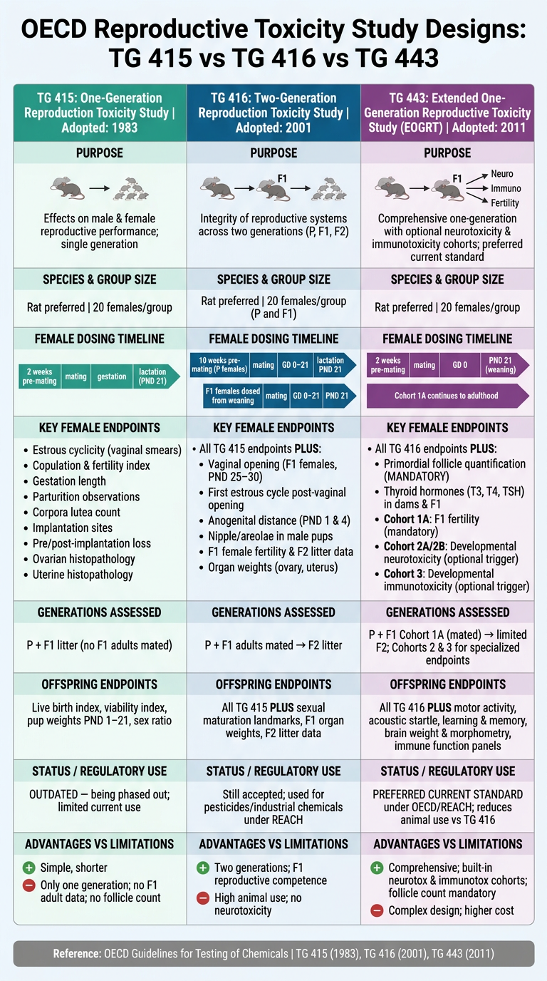
- The oldest and simplest design; females dosed 2 weeks pre-mating through lactation
- Only one generation assessed; no F1 adult mating
- Being phased out - limited current regulatory acceptance
- Adds a full F1 generation of adult females dosed from weaning, mated to produce an F2 litter
- Captures vaginal opening, first estrous cycle, and F1 female fertility
- Still widely used under REACH for industrial chemicals and pesticides
- The current preferred OECD standard - replaces TG 416 for most purposes
- Mandatory primordial follicle quantification and thyroid hormones in dams/F1
- Modular cohort system: Cohort 2 (neurotoxicity) and Cohort 3 (immunotoxicity) can be triggered
- Reduces total animal use vs TG 416 while providing deeper mechanistic data
Create a detailed timeline diagram showing dosing windows for each TG
ls -la /home/daytona/workspace/ 2>/dev/null || mkdir -p /home/daytona/workspace && echo "workspace ready"
mkdir -p /home/daytona/workspace/oecd-timeline && python3 << 'EOF' import matplotlib matplotlib.use('Agg') import matplotlib.pyplot as plt import matplotlib.patches as mpatches from matplotlib.patches import FancyArrowPatch, FancyBboxPatch import matplotlib.patheffects as pe import numpy as np # ── colour palette ────────────────────────────────────────────────────────── C = { 'bg': '#F8F9FC', 'grid': '#E2E6ED', 'teal': '#00897B', 'teal_lt': '#B2DFDB', 'blue': '#1565C0', 'blue_lt': '#BBDEFB', 'purple': '#6A1B9A', 'purple_lt': '#E1BEE7', # phase colours 'premating': '#FF8F00', 'mating': '#F57F17', 'gestation': '#2E7D32', 'lactation': '#1565C0', 'weaning': '#6A1B9A', 'adult': '#AD1457', 'cohort2': '#00838F', 'cohort3': '#558B2F', 'f2': '#E65100', 'necropsy': '#B71C1C', 'white': '#FFFFFF', 'dark': '#1A1A2E', 'subtext': '#4A4A6A', } # ── figure ─────────────────────────────────────────────────────────────────── fig = plt.figure(figsize=(24, 20), facecolor=C['bg']) ax = fig.add_axes([0, 0, 1, 1]) ax.set_xlim(0, 1) ax.set_ylim(0, 1) ax.axis('off') ax.set_facecolor(C['bg']) # ── helpers ─────────────────────────────────────────────────────────────────── def bar(ax, x0, x1, y, h, color, alpha=1.0, radius=0.008, label=None, fontsize=8.5, zorder=3): """Draw a rounded rectangle bar.""" width = x1 - x0 rect = FancyBboxPatch((x0, y - h/2), width, h, boxstyle=f"round,pad=0,rounding_size={radius}", linewidth=0, facecolor=color, alpha=alpha, zorder=zorder) ax.add_patch(rect) if label: mid = (x0 + x1) / 2 ax.text(mid, y, label, ha='center', va='center', fontsize=fontsize, fontweight='bold', color=C['white'], zorder=zorder+1, path_effects=[pe.withStroke(linewidth=1.5, foreground='#00000040')]) def vline(ax, x, y0, y1, color='#888', lw=1, ls='--', zorder=2): ax.plot([x, x], [y0, y1], color=color, linewidth=lw, linestyle=ls, zorder=zorder) def tick_label(ax, x, y, label, fontsize=8, color='#555', ha='center'): ax.text(x, y, label, ha=ha, va='top', fontsize=fontsize, color=color, fontfamily='monospace') def section_header(ax, x, y, w, h, label, color, sub=''): rect = FancyBboxPatch((x, y), w, h, boxstyle="round,pad=0,rounding_size=0.006", linewidth=0, facecolor=color, zorder=4) ax.add_patch(rect) ax.text(x + w/2, y + h*0.62, label, ha='center', va='center', fontsize=14, fontweight='bold', color=C['white'], zorder=5) if sub: ax.text(x + w/2, y + h*0.22, sub, ha='center', va='center', fontsize=9.5, color='#FFFFFFCC', zorder=5) def row_bg(ax, y_center, height, color='#FFFFFF80', zorder=1): rect = FancyBboxPatch((0.01, y_center - height/2), 0.98, height, boxstyle="round,pad=0,rounding_size=0.004", linewidth=0.5, edgecolor='#D0D4DD', facecolor=color, zorder=zorder) ax.add_patch(rect) def annotation(ax, x, y, text, color, fontsize=7.5): ax.text(x, y, text, ha='center', va='bottom', fontsize=fontsize, color=color, fontweight='bold', rotation=0) def side_label(ax, x, y, text, color, fontsize=10): ax.text(x, y, text, ha='right', va='center', fontsize=fontsize, color=color, fontweight='bold') # ── TITLE ───────────────────────────────────────────────────────────────────── ax.text(0.5, 0.975, 'OECD Reproductive Toxicity Test Guidelines', ha='center', va='top', fontsize=22, fontweight='bold', color=C['dark']) ax.text(0.5, 0.953, 'Dosing Windows & Study Timeline Comparison · TG 415 | TG 416 | TG 443 (EOGRT)', ha='center', va='top', fontsize=13, color=C['subtext']) # thin separator line ax.plot([0.03, 0.97], [0.942, 0.942], color='#C0C8D8', linewidth=1.5) # ── LEGEND ──────────────────────────────────────────────────────────────────── legend_y = 0.928 legend_items = [ ('Pre-mating dosing', C['premating']), ('Mating period', C['mating']), ('Gestation (GD 0–21)', C['gestation']), ('Lactation (PND 0–21)',C['lactation']), ('Post-weaning / Adult',C['adult']), ('F2 Litter phase', C['f2']), ('Cohort 2 – Neuro', C['cohort2']), ('Cohort 3 – Immuno', C['cohort3']), ('Necropsy ✚', C['necropsy']), ] lx = 0.04 for label, col in legend_items: rect = FancyBboxPatch((lx, legend_y - 0.010), 0.022, 0.016, boxstyle="round,pad=0,rounding_size=0.003", linewidth=0, facecolor=col, zorder=5) ax.add_patch(rect) ax.text(lx + 0.025, legend_y - 0.002, label, va='center', fontsize=8, color=C['dark']) lx += 0.107 # ── TIMELINE X-AXIS SETUP ──────────────────────────────────────────────────── # We map study days onto a common relative axis # Origin = Start of Pre-mating dosing (Day 0 of study) # All three TGs aligned at GD 0 (conception) for visual clarity # Key day markers (relative to start of pre-mating dosing): # TG 415: Day 0=pre-mating start; Day 14=GD0; Day 35=GD21(birth); Day 56=PND21(wean/necropsy) # TG 416: Day 0=P pre-mating; Day 70=P GD0; Day 91=P GD21; Day 112=F1PND21(wean) # F1 females then dosed from Day 112; F1 mating ~Day 182; F1 GD0 ~Day 182 # F1 GD21 ~Day 203; F2 PND21 ~Day 224 (necropsy) # TG 443: Day 0=pre-mating; Day 14=GD0; Day 35=GD21; Day 56=PND21 # Cohort 1A continues to ~Day 126 (adult mating) # Cohort 2 continues to ~Day 140 (neurotox done) # Cohort 3 continues to ~Day 140 (immunotox done) # Global x range covers 0..240 days DAY_MIN = -14 # 2 weeks before pre-mating for context DAY_MAX = 240 def d2x(day): """Convert study day to axes x coordinate (0.09 to 0.97).""" return 0.09 + (day - DAY_MIN) / (DAY_MAX - DAY_MIN) * 0.88 # ── X-AXIS (shared timeline) ────────────────────────────────────────────────── AXIS_Y = 0.082 ax.annotate('', xy=(d2x(DAY_MAX)+0.005, AXIS_Y), xytext=(d2x(DAY_MIN)-0.005, AXIS_Y), arrowprops=dict(arrowstyle='->', color=C['dark'], lw=2), zorder=6) # day tick marks at key milestones tick_days = { -14: '-14', 0: '0\n(Pre-mating\nstart)', 14: 'GD 0\n(±14)', 35: 'GD 21\n(Birth)', 56: 'PND 21\n(Wean)', 70: 'Day 70\n(P GD 0\nTG416)', 91: 'Day 91\n(P Birth\nTG416)', 112: 'Day 112\n(F1 Wean\nTG416)', 126: 'Day 126\n(F1 Adult)', 182: 'Day 182\n(F1 GD 0\nTG416)', 203: 'Day 203\n(F2 Birth)', 224: 'Day 224\n(F2 Wean\nNecropsy)', } for day, lbl in tick_days.items(): tx = d2x(day) ax.plot([tx, tx], [AXIS_Y - 0.008, AXIS_Y + 0.008], color=C['dark'], lw=1.2, zorder=6) ax.text(tx, AXIS_Y - 0.012, lbl, ha='center', va='top', fontsize=6.5, color=C['subtext'], linespacing=1.3) ax.text(d2x(DAY_MAX)+0.012, AXIS_Y, 'Study Days', ha='left', va='center', fontsize=9, color=C['dark'], fontweight='bold') # ── SECTION HEADERS (TG labels on left) ────────────────────────────────────── # Row Y centers (from top) Y_TG415_H = 0.86 # TG 415 section header top Y_TG415_P = 0.80 # TG 415 P-generation row Y_TG415_F1 = 0.74 # TG 415 F1 litter row Y_TG416_H = 0.64 Y_TG416_P = 0.58 Y_TG416_F1 = 0.52 Y_TG416_F2 = 0.46 Y_TG443_H = 0.36 Y_TG443_P = 0.30 Y_TG443_C1A = 0.24 Y_TG443_C2 = 0.18 Y_TG443_C3 = 0.12 BAR_H = 0.030 HEADER_H = 0.030 # ── row backgrounds ─────────────────────────────────────────────────────────── for yc in [Y_TG415_P, Y_TG415_F1, Y_TG416_P, Y_TG416_F1, Y_TG416_F2, Y_TG443_P, Y_TG443_C1A, Y_TG443_C2, Y_TG443_C3]: row_bg(ax, yc, BAR_H + 0.018) # ── TG 415 SECTION ─────────────────────────────────────────────────────────── section_header(ax, 0.01, Y_TG415_H - 0.002, 0.07, HEADER_H + 0.008, 'OECD TG 415', C['teal'], 'One-Generation (1983)') ax.plot([0.01, 0.97], [Y_TG415_H - 0.004, Y_TG415_H - 0.004], color=C['teal'], linewidth=1.0, alpha=0.4) # P generation row label side_label(ax, 0.085, Y_TG415_P, 'P ♀ (Parent)', C['teal'], 10) # Pre-mating: Day 0–14 bar(ax, d2x(0), d2x(14), Y_TG415_P, BAR_H, C['premating'], label='Pre-mating\n14 days') annotation(ax, d2x(7), Y_TG415_P + BAR_H/2 + 0.008, '2 oestrous cycles', C['premating']) # Mating: Day 14–19 bar(ax, d2x(14), d2x(19), Y_TG415_P, BAR_H, C['mating'], label='Mat.') # Gestation: Day 19–40 (GD 0–21) bar(ax, d2x(19), d2x(40), Y_TG415_P, BAR_H, C['gestation'], label='Gestation\nGD 0–21') # Lactation: Day 40–61 (PND 0–21) bar(ax, d2x(40), d2x(61), Y_TG415_P, BAR_H, C['lactation'], label='Lactation\nPND 0–21') # Necropsy marker vline(ax, d2x(61), Y_TG415_P - BAR_H/2 - 0.005, Y_TG415_P + BAR_H/2 + 0.005, C['necropsy'], lw=2.5, ls='-') annotation(ax, d2x(61), Y_TG415_P + BAR_H/2 + 0.008, '✚ Necropsy PND 21', C['necropsy']) # F1 litter row side_label(ax, 0.085, Y_TG415_F1, 'F1 Litter', C['teal'], 10) bar(ax, d2x(40), d2x(61), Y_TG415_F1, BAR_H, C['lactation'], alpha=0.55, label='F1 Pups\nPND 0–21') annotation(ax, d2x(50), Y_TG415_F1 - BAR_H/2 - 0.012, 'Live birth index · Viability index · Pup weights · Sex ratio', C['subtext'], fontsize=7.5) # Necropsy marker F1 vline(ax, d2x(61), Y_TG415_F1 - BAR_H/2 - 0.005, Y_TG415_F1 + BAR_H/2 + 0.005, C['necropsy'], lw=2.5, ls='-') # Status badge rect = FancyBboxPatch((d2x(70), Y_TG415_H - 0.016), 0.13, 0.022, boxstyle="round,pad=0,rounding_size=0.004", linewidth=0, facecolor='#FF6F00', zorder=6) ax.add_patch(rect) ax.text(d2x(70) + 0.065, Y_TG415_H - 0.006, '⚠ OUTDATED — limited current regulatory use', ha='center', va='center', fontsize=8.5, color=C['white'], fontweight='bold', zorder=7) # ── TG 416 SECTION ─────────────────────────────────────────────────────────── section_header(ax, 0.01, Y_TG416_H - 0.002, 0.07, HEADER_H + 0.008, 'OECD TG 416', C['blue'], 'Two-Generation (2001)') ax.plot([0.01, 0.97], [Y_TG416_H - 0.004, Y_TG416_H - 0.004], color=C['blue'], linewidth=1.0, alpha=0.4) # P generation side_label(ax, 0.085, Y_TG416_P, 'P ♀ (Parental)', C['blue'], 10) # Pre-mating: 10 weeks = 70 days bar(ax, d2x(0), d2x(70), Y_TG416_P, BAR_H, C['premating'], label='Pre-mating 70 days (10 wks)') annotation(ax, d2x(35), Y_TG416_P + BAR_H/2 + 0.008, 'folliculogenesis + spermatogenesis cycle', C['premating']) bar(ax, d2x(70), d2x(75), Y_TG416_P, BAR_H, C['mating'], label='Mat.') bar(ax, d2x(75), d2x(96), Y_TG416_P, BAR_H, C['gestation'], label='Gestation GD 0–21') bar(ax, d2x(96), d2x(117), Y_TG416_P, BAR_H, C['lactation'], label='Lactation PND 0–21') vline(ax, d2x(117), Y_TG416_P - BAR_H/2, Y_TG416_P + BAR_H/2 + 0.005, C['necropsy'], lw=2.5, ls='-') annotation(ax, d2x(117), Y_TG416_P + BAR_H/2 + 0.008, '✚ P Necropsy', C['necropsy']) # F1 females side_label(ax, 0.085, Y_TG416_F1, 'F1 ♀ (Daughters)', C['blue'], 10) # F1 dosed from weaning (Day 117) pre-mating 14 days; mating Day 131; GD0 Day 136; Birth Day 157; Wean/necropsy Day 178 bar(ax, d2x(117), d2x(131), Y_TG416_F1, BAR_H, C['premating'], label='Pre-mating 14d') annotation(ax, d2x(117), Y_TG416_F1 + BAR_H/2 + 0.008, 'Vaginal opening monitored\nfrom PND 25–30', C['premating'], 7.5) bar(ax, d2x(131), d2x(136), Y_TG416_F1, BAR_H, C['mating'], label='Mat.') bar(ax, d2x(136), d2x(157), Y_TG416_F1, BAR_H, C['gestation'], label='Gestation GD 0–21') bar(ax, d2x(157), d2x(178), Y_TG416_F1, BAR_H, C['lactation'], label='Lactation PND 0–21') vline(ax, d2x(178), Y_TG416_F1 - BAR_H/2, Y_TG416_F1 + BAR_H/2 + 0.005, C['necropsy'], lw=2.5, ls='-') annotation(ax, d2x(178), Y_TG416_F1 + BAR_H/2 + 0.008, '✚ F1 Necropsy', C['necropsy']) # F2 litter side_label(ax, 0.085, Y_TG416_F2, 'F2 Litter', C['blue'], 10) bar(ax, d2x(157), d2x(178), Y_TG416_F2, BAR_H, C['f2'], alpha=0.75, label='F2 Pups PND 0–21') annotation(ax, d2x(167), Y_TG416_F2 - BAR_H/2 - 0.012, 'Live birth · viability · pup weights · sex ratio · organ weights · AGD', C['subtext'], 7.5) vline(ax, d2x(178), Y_TG416_F2 - BAR_H/2, Y_TG416_F2 + BAR_H/2 + 0.005, C['necropsy'], lw=2.5, ls='-') # Status badge TG 416 rect2 = FancyBboxPatch((d2x(185), Y_TG416_H - 0.016), 0.14, 0.022, boxstyle="round,pad=0,rounding_size=0.004", linewidth=0, facecolor=C['blue'], zorder=6) ax.add_patch(rect2) ax.text(d2x(185) + 0.070, Y_TG416_H - 0.006, '✔ Still accepted | REACH / pesticides / industrial chemicals', ha='center', va='center', fontsize=8.5, color=C['white'], fontweight='bold', zorder=7) # ── TG 443 SECTION ─────────────────────────────────────────────────────────── section_header(ax, 0.01, Y_TG443_H - 0.002, 0.07, HEADER_H + 0.008, 'OECD TG 443', C['purple'], 'EOGRT — Extended One-Gen (2011)') ax.plot([0.01, 0.97], [Y_TG443_H - 0.004, Y_TG443_H - 0.004], color=C['purple'], linewidth=1.0, alpha=0.4) # P generation side_label(ax, 0.085, Y_TG443_P, 'P ♀ (Parental)', C['purple'], 10) bar(ax, d2x(0), d2x(14), Y_TG443_P, BAR_H, C['premating'], label='Pre-mating 14d') annotation(ax, d2x(7), Y_TG443_P + BAR_H/2 + 0.008, '≥2 oestrous cycles · follicle count · T3/T4/TSH', C['premating']) bar(ax, d2x(14), d2x(19), Y_TG443_P, BAR_H, C['mating'], label='Mat.') bar(ax, d2x(19), d2x(40), Y_TG443_P, BAR_H, C['gestation'], label='Gestation GD 0–21') bar(ax, d2x(40), d2x(61), Y_TG443_P, BAR_H, C['lactation'], label='Lactation PND 0–21') vline(ax, d2x(61), Y_TG443_P - BAR_H/2, Y_TG443_P + BAR_H/2 + 0.005, C['necropsy'], lw=2.5, ls='-') annotation(ax, d2x(61), Y_TG443_P + BAR_H/2 + 0.008, '✚ P Necropsy\nPrimordial follicle count (MANDATORY)', C['necropsy'], 7) # Cohort 1A side_label(ax, 0.085, Y_TG443_C1A, 'Cohort 1A ♀\n(F1 Fertility)', C['purple'], 9) bar(ax, d2x(61), d2x(75), Y_TG443_C1A, BAR_H, C['adult'], label='Post-wean growth') annotation(ax, d2x(61), Y_TG443_C1A + BAR_H/2 + 0.008, 'Vaginal opening · 1st estrous · AGD monitored', C['adult']) bar(ax, d2x(75), d2x(110), Y_TG443_C1A, BAR_H, C['adult'], alpha=0.7, label='Adult pre-mating (≥10 wks)') bar(ax, d2x(110), d2x(115), Y_TG443_C1A, BAR_H, C['mating'], label='Mat.') bar(ax, d2x(115), d2x(136), Y_TG443_C1A, BAR_H, C['gestation'], label='GD 0–21') bar(ax, d2x(136), d2x(157), Y_TG443_C1A, BAR_H, C['f2'], label='F2 Litter PND 0–21') vline(ax, d2x(157), Y_TG443_C1A - BAR_H/2, Y_TG443_C1A + BAR_H/2 + 0.005, C['necropsy'], lw=2.5, ls='-') annotation(ax, d2x(157), Y_TG443_C1A + BAR_H/2 + 0.008, '✚ Necropsy', C['necropsy']) # Cohort 2 (Developmental Neurotoxicity — triggered) side_label(ax, 0.085, Y_TG443_C2, 'Cohort 2\n(DNT — if triggered)', C['cohort2'], 9) bar(ax, d2x(40), d2x(61), Y_TG443_C2, BAR_H, C['lactation'], alpha=0.5, label='PND 0–21') bar(ax, d2x(61), d2x(140), Y_TG443_C2, BAR_H, C['cohort2'], alpha=0.85, label='Neurobehavioral endpoints PND 21 → PND ~77') annotation(ax, d2x(100), Y_TG443_C2 + BAR_H/2 + 0.008, 'Motor activity · Acoustic startle · Learning & memory · Brain morphometry', C['cohort2']) vline(ax, d2x(140), Y_TG443_C2 - BAR_H/2, Y_TG443_C2 + BAR_H/2 + 0.005, C['necropsy'], lw=2.5, ls='-') annotation(ax, d2x(140), Y_TG443_C2 + BAR_H/2 + 0.008, '✚', C['necropsy']) # Cohort 3 (Developmental Immunotoxicity — triggered) side_label(ax, 0.085, Y_TG443_C3, 'Cohort 3\n(DIT — if triggered)', C['cohort3'], 9) bar(ax, d2x(40), d2x(61), Y_TG443_C3, BAR_H, C['lactation'], alpha=0.5, label='PND 0–21') bar(ax, d2x(61), d2x(126), Y_TG443_C3, BAR_H, C['cohort3'], alpha=0.85, label='Immunological assessments PND 21 → PND ~56') annotation(ax, d2x(90), Y_TG443_C3 - BAR_H/2 - 0.012, 'Lymphocyte subsets · NK cell activity · T-cell dependent antibody response', C['subtext'], 7.5) vline(ax, d2x(126), Y_TG443_C3 - BAR_H/2, Y_TG443_C3 + BAR_H/2 + 0.005, C['necropsy'], lw=2.5, ls='-') annotation(ax, d2x(126), Y_TG443_C3 + BAR_H/2 + 0.008, '✚', C['necropsy']) # Status badge TG 443 rect3 = FancyBboxPatch((d2x(165), Y_TG443_H - 0.016), 0.165, 0.022, boxstyle="round,pad=0,rounding_size=0.004", linewidth=0, facecolor=C['purple'], zorder=6) ax.add_patch(rect3) ax.text(d2x(165) + 0.083, Y_TG443_H - 0.006, '★ PREFERRED CURRENT STANDARD | OECD / REACH / Regulatory default', ha='center', va='center', fontsize=8.5, color=C['white'], fontweight='bold', zorder=7) # ── vertical milestone lines across entire chart ────────────────────────────── milestones = [ (d2x(0), 'Day 0\nPre-mating\nbegins', '#FF8F00'), (d2x(14), 'GD 0\n(≈Day 14)', '#2E7D32'), (d2x(35), 'GD 21\nBirth', '#2E7D32'), (d2x(61), 'PND 21\nWeaning', '#1565C0'), ] for mx, mlabel, mcol in milestones: ax.plot([mx, mx], [0.095, Y_TG415_H - 0.01], color=mcol, linewidth=1.2, linestyle=':', alpha=0.5, zorder=1) # ── bottom footer ───────────────────────────────────────────────────────────── ax.plot([0.03, 0.97], [0.068, 0.068], color='#C0C8D8', linewidth=1.2) ax.text(0.5, 0.058, 'GD = Gestational Day · PND = Postnatal Day · Mat. = Mating · AGD = Anogenital Distance · DNT = Developmental Neurotoxicity · DIT = Developmental Immunotoxicity', ha='center', va='center', fontsize=8, color=C['subtext']) ax.text(0.5, 0.044, 'Reference: OECD Guidelines for Testing of Chemicals | TG 415 (1983) · TG 416 (2001) · TG 443 (2011) · Bars represent FEMALE dosing windows', ha='center', va='center', fontsize=8, color=C['subtext']) # outer border border = FancyBboxPatch((0.005, 0.005), 0.990, 0.990, boxstyle="round,pad=0,rounding_size=0.01", linewidth=2, edgecolor='#B0BAD0', facecolor='none', zorder=10) ax.add_patch(border) # ── save ────────────────────────────────────────────────────────────────────── out = '/home/daytona/workspace/oecd-timeline/OECD_TG_Timeline_Diagram.png' fig.savefig(out, dpi=180, bbox_inches='tight', facecolor=C['bg']) plt.close() print(f"Saved: {out}") EOF
ls -lh /home/daytona/workspace/oecd-timeline/OECD_TG_Timeline_Diagram.png
OECD TG Timeline Diagram
Image · PNG
TG 415 (Teal - top section)
- P female row: Orange pre-mating bar (14 days, 2 estrous cycles) → mating → green gestation (GD 0-21) → blue lactation (PND 0-21) → red necropsy marker
- F1 litter row: Shows pup monitoring PND 0-21; annotated with live birth index, viability index, pup weights, sex ratio
- Status badge: ⚠ OUTDATED - limited current regulatory use
TG 416 (Blue - middle section)
- P female row: 70-day pre-mating bar (10 weeks for full folliculogenesis) → mating → gestation → lactation → necropsy
- F1 daughters row: Dosed from weaning (Day 117) → pre-mating with vaginal opening monitoring → mating → gestation → lactation → necropsy
- F2 litter row: PND 0-21 with AGD, organ weights annotated
- Status badge: ✔ Still accepted - REACH / pesticides / industrial chemicals
TG 443 EOGRT (Purple - bottom section)
- P female row: Pre-mating with mandatory primordial follicle count + T3/T4/TSH annotation → gestation → lactation → necropsy
- Cohort 1A (F1 fertility): Post-wean growth → adult pre-mating → mating → gestation → F2 litter → necropsy
- Cohort 2 (DNT - triggered): Extends from PND 21 to ~Day 140 with motor activity, startle, learning/memory, brain morphometry
- Cohort 3 (DIT - triggered): Extends to ~Day 126 with lymphocyte subsets, NK cell activity, T-cell antibody response
- Status badge: ★ PREFERRED CURRENT STANDARD