Explain to me Echocardiography in detail from basics all the way to advanced in detail with reference from the echo manual and Braunwald with all the relevant images
Reading File
Finding Sources
Finding Sources
Finding Sources
Finding Sources
Reading File
Finding Sources
Finding Sources
Reading File
Finding Sources
Reading File
Reading File
Reading File
Reading File
Reading File
Reading File
Reading File
Loading Image
Loading Image
Loading Image
Loading Image
Reading File
Loading Image
Reading File
Loading Image
Loading Image
I now have all the foundational content, images, and advanced material needed. Let me now compose the comprehensive, detailed echocardiography guide drawing from the Textbook of Clinical Echocardiography (Echo Manual) and Braunwald's Heart Disease.
Echocardiography: From Basics to Advanced
Primary references: Textbook of Clinical Echocardiography (Otto et al., 9780323882088) and Braunwald's Heart Disease (9780323722193)
PART 1: ULTRASOUND PHYSICS - THE FOUNDATION
Sound Waves and Ultrasound
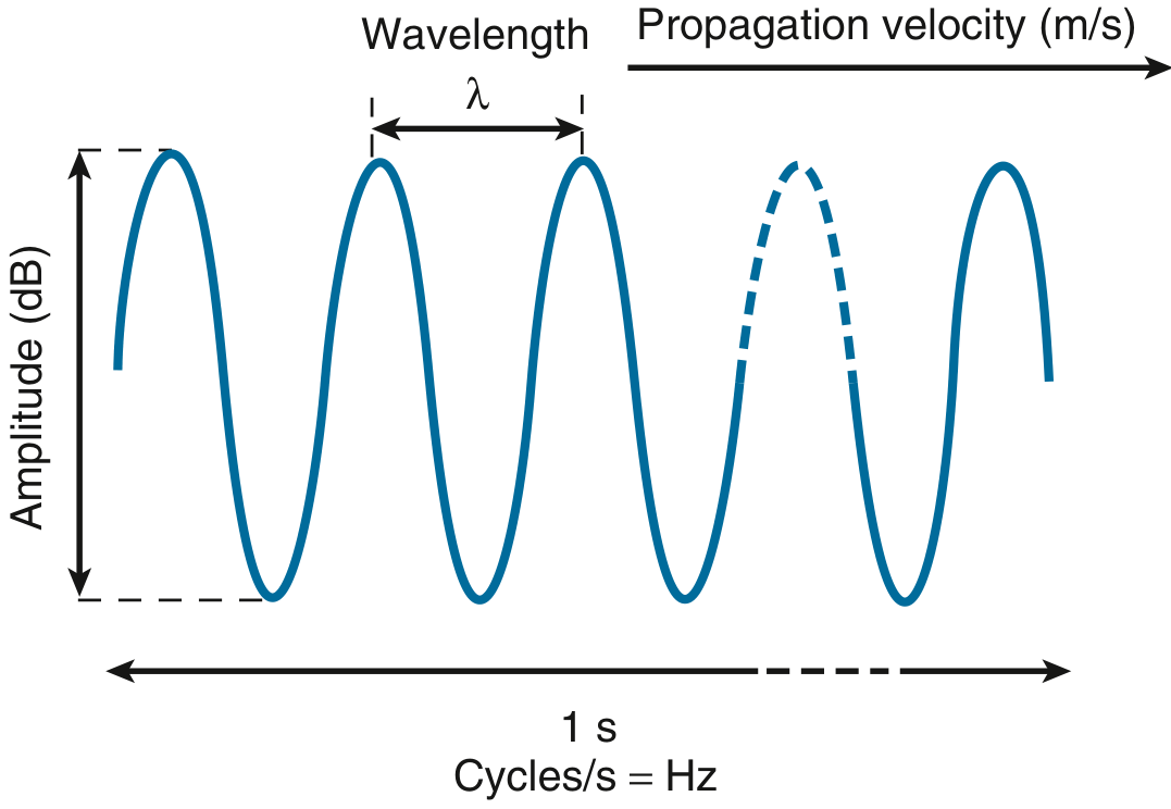
Sound waves are mechanical vibrations that induce alternate rarefaction and compression of any physical medium through which they pass. Four key properties define them:
| Property | Unit | Clinical Relevance |
|---|---|---|
| Frequency | Hertz (Hz) = cycles/second | Determines resolution vs. penetration |
| Velocity of propagation (c) | m/s | ~1540 m/s in soft tissue |
| Wavelength (λ) | mm | λ = c/f |
| Amplitude | Decibels (dB) | Signal strength |
Diagnostic ultrasound uses frequencies between 1 and 20 MHz - well above the human hearing range of 20 Hz to 20 kHz. The critical formula:
λ (mm) = 1.54 / f (MHz)
For a 5 MHz transducer: λ = 1540/5,000,000 = 0.308 mm
This leads to a fundamental trade-off:
- Higher frequency = shorter wavelength = better resolution but less penetration
- Lower frequency = longer wavelength = deeper penetration but poorer resolution
Image resolution is no better than 1-2 wavelengths (~1 mm), and penetration depth is directly related to wavelength.
Ultrasound-Tissue Interaction
When an ultrasound beam travels through the body, four interactions occur:
1. Reflection - When the beam strikes an interface between two tissues with different acoustic impedance (Z = density × propagation velocity), part of the energy is reflected back to the transducer. Strong reflectors (specular reflectors) include valve leaflets and endocardial surfaces when the beam is perpendicular to them. The percentage of reflected energy = [(Z2 - Z1)/(Z2 + Z1)]²
2. Scattering - Occurs when the beam hits structures smaller than the wavelength (e.g., red blood cells, myocardial fibers). Scattering is the basis of tissue characterization and Doppler detection of blood flow. Scattered signals return from all angles (unlike specular reflection), so they are detectable even when the beam is not perfectly perpendicular.
3. Refraction - Bending of the ultrasound beam when it crosses an interface at an oblique angle with different propagation velocities. This is a source of imaging artifacts (misregistration of depth).
4. Attenuation - Progressive decrease in signal amplitude with depth. Attenuation increases with:
- Higher frequency
- Denser tissues
- Greater depth
Attenuation coefficient α describes loss in dB/cm/MHz. In soft tissue ≈ 0.5 dB/cm/MHz.
Transducers
The piezoelectric crystal is the key component. It converts electrical energy to mechanical (acoustic) energy during transmission and mechanical energy back to electrical energy during reception. This dual function makes it both the "speaker" and "microphone" of the system.
Modern transducers are phased array types containing 64-256 or more individual elements that can be electronically steered and focused:
- Electronic beam steering: elements are fired in sequence with tiny delays, steering the beam across the image sector
- Electronic focusing: delays are applied to create constructive interference at the focal zone
Key transducer types in cardiology:
| Type | Frequency | Use |
|---|---|---|
| Phased array (transthoracic) | 2-5 MHz | Standard TTE |
| Transesophageal (TEE) | 5-7 MHz | High-res posterior structures |
| Intracardiac (ICE) | 5-10 MHz | Catheterization lab |
| Hand-held | 2-4 MHz | Point-of-care |
Resolution has two components:
- Axial resolution (along beam direction) = determined by pulse length = 1-2 wavelengths (~0.5-1 mm at 3-5 MHz)
- Lateral resolution (perpendicular to beam) = beam width at focal zone = poorer than axial, typically 2-3 mm
PART 2: IMAGING MODALITIES
M-Mode Echocardiography
The earliest cardiac ultrasound modality. A single crystal emits a single line of ultrasound, and returning signals are displayed with time on the X-axis and depth on the Y-axis, creating a "motion" (M) record.
Pulse repetition frequency (PRF) in M-mode is ~1800 times/second - far higher than 2D, which makes M-mode exquisitely sensitive to rapid motion. At 20 cm depth, only 0.26 ms is needed per pulse cycle.
Classic M-mode recordings:
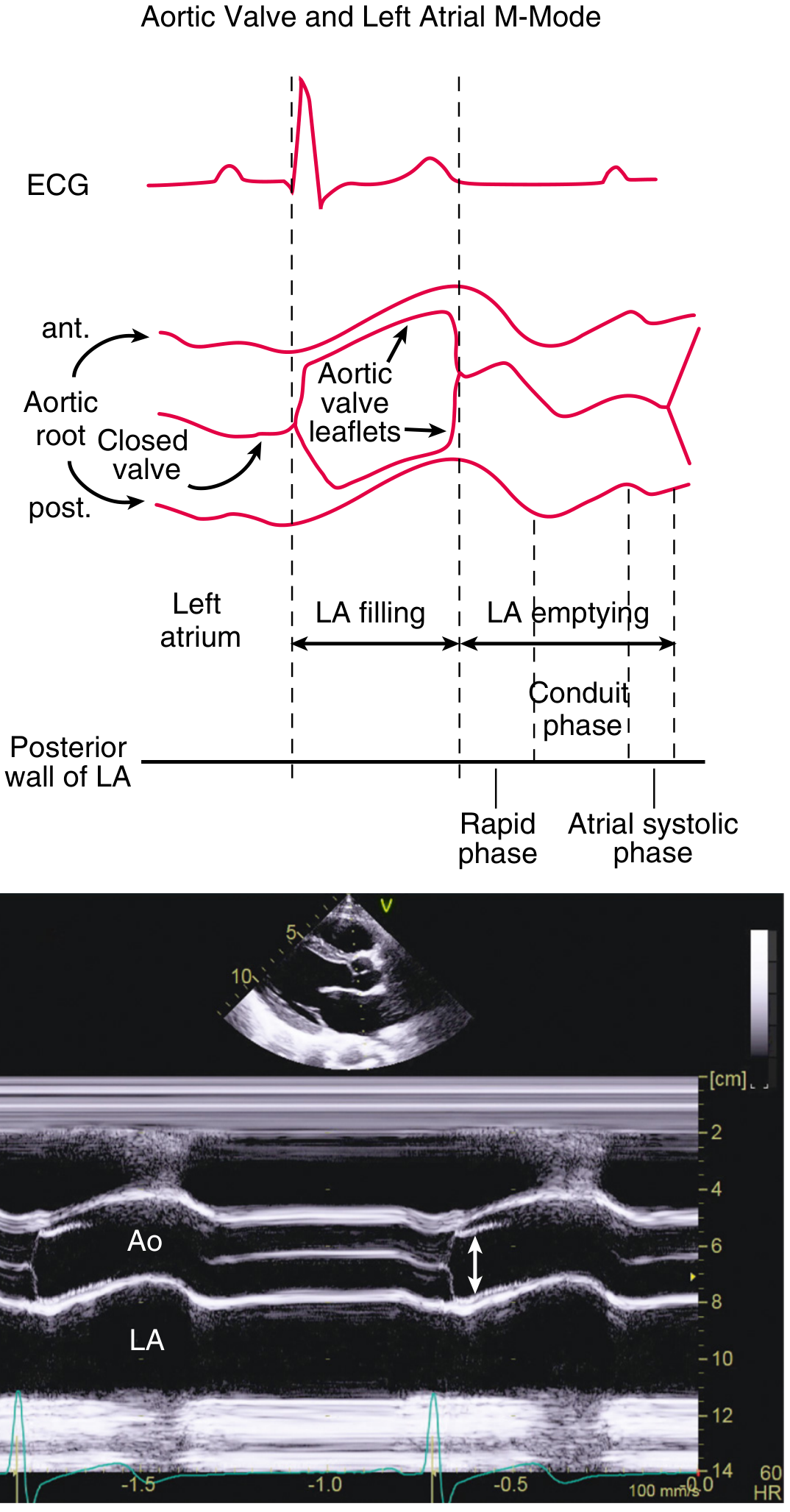
Aortic valve and LA:
- Aortic leaflets open in systole to form a "box" shape
- Left atrial dimension measured at end-systole (largest)
- Normal aortic root dimension: ≤ 2.1 cm/m² at sinuses
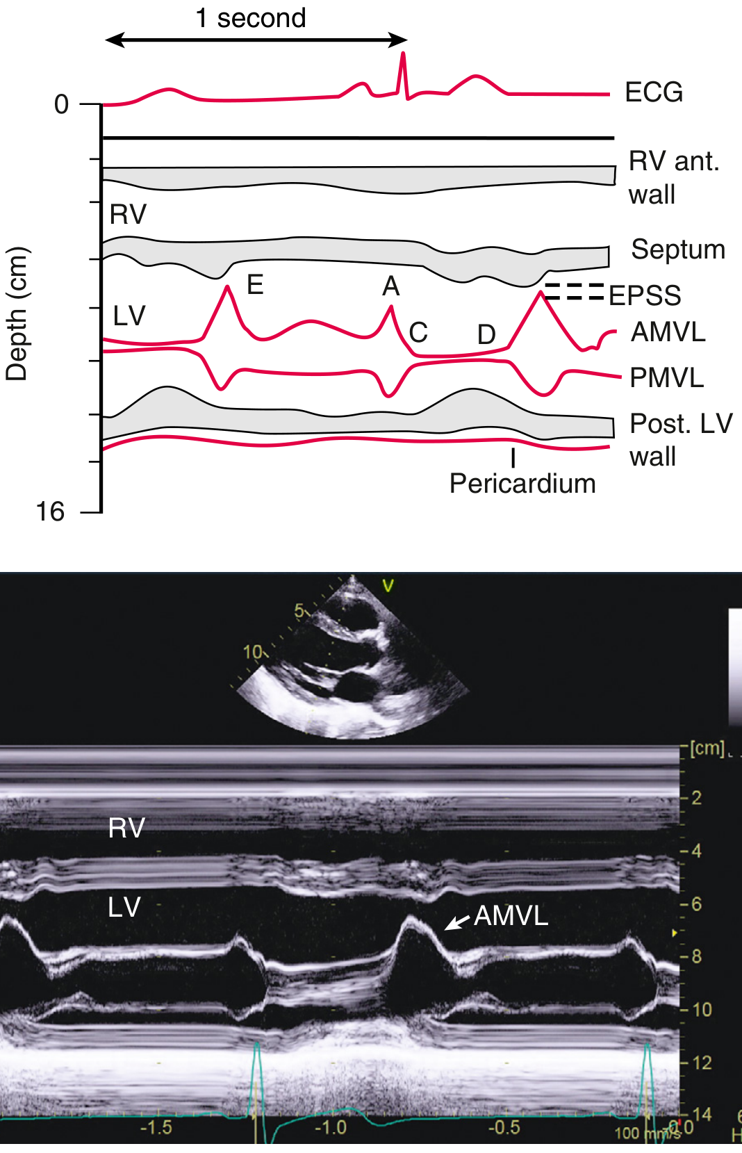
Mitral valve (the most informative M-mode):
- E-point = maximum early diastolic anterior leaflet excursion
- A-point = late diastolic peak (atrial contraction)
- EPSS (E-point to septal separation): normally < 7 mm. Increased EPSS indicates LV dilation, systolic dysfunction, or AR
- B-bump (AC shoulder): seen when LV end-diastolic pressure is elevated
- Fine fluttering of anterior leaflet: pathognomonic of aortic regurgitation
LV M-mode:
- Measured at papillary muscle level, perpendicular to LV long axis
- Provides: IVSd, LVIDd, LVPWd, IVSs, LVIDs, LVPWs
- Used to calculate fractional shortening (FS): FS = (LVIDd - LVIDs)/LVIDd × 100%
- Normal FS: 25-45%
2D Echocardiography
Image production: The phased array transducer electronically sweeps the beam across the image sector. For each scan line, a short pulse is emitted and the returning signal processed. Key parameters:
- PRF = limited by time for ultrasound to reach maximum depth and return
- Frame rate must be ≥ 30 frames/second for cardiac applications (33 ms/frame)
- A 20 cm depth at 128 scan lines = 33 ms per frame
Signal processing chain:
- Signal amplification
- Time-gain compensation (TGC): compensates for increasing attenuation with depth
- Compression/dynamic range adjustment
- Gray-scale mapping
- Digital scan conversion and display
Instrument settings to optimize:
- Frequency: balance resolution vs. penetration
- Gain: overall amplitude; too high = "white out"; too low = drop-out
- TGC sliders: adjust near- and far-field gain independently
- Depth: use minimum depth that shows all structures of interest
- Focus: set at level of main structure of interest
- Harmonic imaging: transmit at f₀, receive at 2f₀ - dramatically reduces artifact, improves endocardial definition
Common 2D artifacts:
| Artifact | Cause | Example |
|---|---|---|
| Reverberation | Multiple round-trip reflections | "Extra lines" in LA near prosthetic valves |
| Side-lobe artifact | Off-axis beam reflections | Apparent "masses" in cardiac chambers |
| Near-field clutter | High-amplitude near-field noise | Masks structures immediately under transducer |
| Shadowing | Dense structure absorbs beam | Behind calcified valves or pericardial effusions |
| Refraction | Velocity change at interface | Image duplication |
Standard Imaging Windows and Views
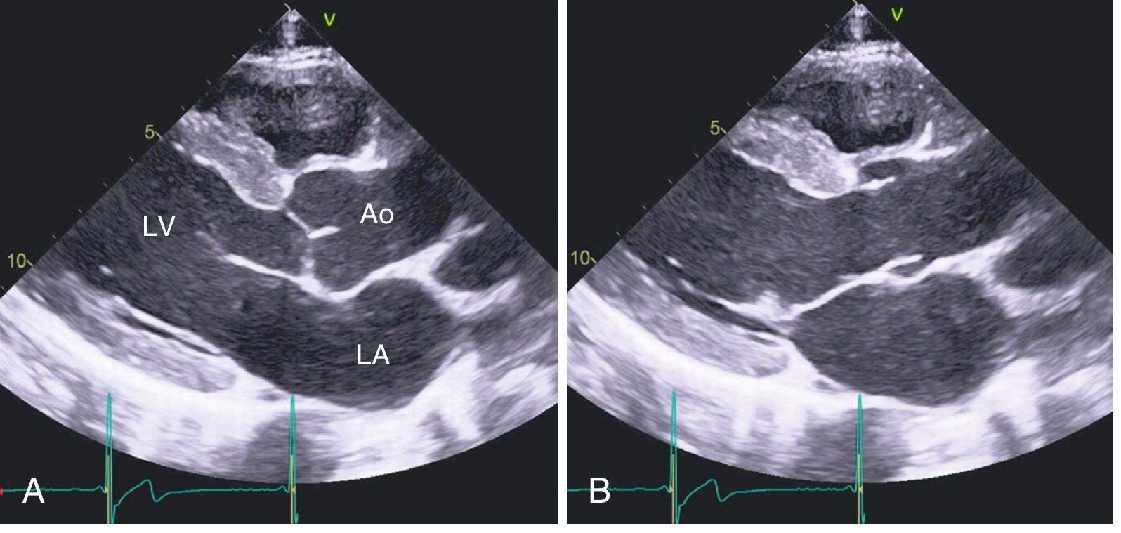
Parasternal Long-Axis View (PLAX):
Shows LV, MV, AV, LA, aortic root, RVOT. The reference view for aortic root measurements.
Normal PLAX anatomy:
- Anterior: RV outflow tract
- Posterior: left atrium
- Aortic valve: right coronary cusp (anterior) and non-coronary cusp (posterior)
- Mitral valve: anterior and posterior leaflets
- Intervalvular fibrosa: fibrous continuity between AV and anterior MV leaflet
Parasternal Short-Axis Views (PSAX):
Rotate 90° clockwise from PLAX. Multiple levels:
- Aortic valve level: "Mercedes-Benz" sign of tri-leaflet AV; TV, PV, RV, RA, PA visible; RVOT; best view for AV planimetry
- Mitral valve level: "fish-mouth" MV opening; used for MVA planimetry in MS
- Papillary muscle level: standard for LV segmental analysis; 2 papillary muscles at 4 and 8 o'clock
- Apical level: circular LV; true apex
Apical Views:
Transducer at cardiac apex; LV apex closest to transducer.
- Apical 4-chamber (A4C): Both ventricles and atria; TV and MV; IAS, IVS; lateral and septal walls; LV apex
- Apical 5-chamber (A5C): Tilt anteriorly to include AV and LVOT - essential for Doppler of LVOT
- Apical 2-chamber (A2C): Rotate ~60° from A4C; inferior and anterior walls only
- Apical 3-chamber / Long-axis (A3C): ~120° from A4C; posterior and anterior walls; AV, MV; similar to PLAX but from apex
Subcostal Views:
- 4-chamber: IAS clearly perpendicular to beam - best view to evaluate ASD (avoid false dropout in apical view)
- Short axis: RVFW; IVS respiratory variation
- IVC: measure IVC diameter for RA pressure estimation
Suprasternal Notch:
- Long-axis view of aortic arch, branch vessels
- CW Doppler for coarctation assessment
3D Echocardiography
Transthoracic and TEE 3D systems use matrix array transducers with thousands of elements to acquire pyramidal volumetric datasets. Modes include:
- Real-time (live) 3D: narrow pyramidal volume, immediate display
- Full-volume acquisition: wide pyramidal dataset stitched from 4-7 cardiac cycles (requires regular rhythm and breath-hold)
- Zoom mode: focused 3D view of a specific structure (e.g., MV, AV)
- Color Doppler 3D: combines full-volume with color flow
Clinical applications of 3D echo:
- LV volumes and EF: more accurate than 2D (avoids geometric assumptions); validated against CMR
- Mitral valve: comprehensive leaflet anatomy; key for surgical planning in MR, for guiding TEER (MitraClip)
- Aortic valve: annulus sizing for TAVR
- ASD/PFO characterization: en-face view of septum
- Guidance of structural interventions: real-time 3D TEE for TAVR, MitraClip, Watchman implantation
As Braunwald notes: "Three-dimensional imaging...allows direct imaging of the orifice area using three-dimensional imaging" for aortic stenosis assessment, and provides superior geometric accuracy for LV volumes.
PART 3: DOPPLER ECHOCARDIOGRAPHY
The Doppler Principle and Equation
The Doppler effect: when sound is reflected from a moving target (red blood cells), the returned frequency is shifted relative to the transmitted frequency. Blood moving toward the transducer increases the returned frequency; blood moving away decreases it.
The Doppler equation mathematically defines this:
$$V = \frac{c \cdot (F_S - F_T)}{2 \cdot F_T \cdot \cos\theta}$$
Where:
- V = blood flow velocity (m/s)
- c = speed of sound in blood (~1540 m/s)
- F_S = backscattered (received) frequency
- F_T = transmitted frequency
- θ = angle between ultrasound beam and blood flow direction
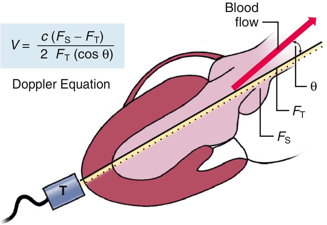
Critical clinical implication of the angle:
- At θ = 0° (parallel): cos θ = 1, no correction needed - ideal
- At θ = 20°: cos θ = 0.94 → only 6% underestimation - acceptable
- At θ = 60°: cos θ = 0.5 → 50% underestimation - clinically significant
- At θ = 90° (perpendicular): cos θ = 0 → no Doppler signal detected
The key rule: always align the Doppler beam as parallel as possible to blood flow. Angle "correction" is NOT used in cardiac Doppler because the true 3D direction of flow cannot be determined from a 2D image.
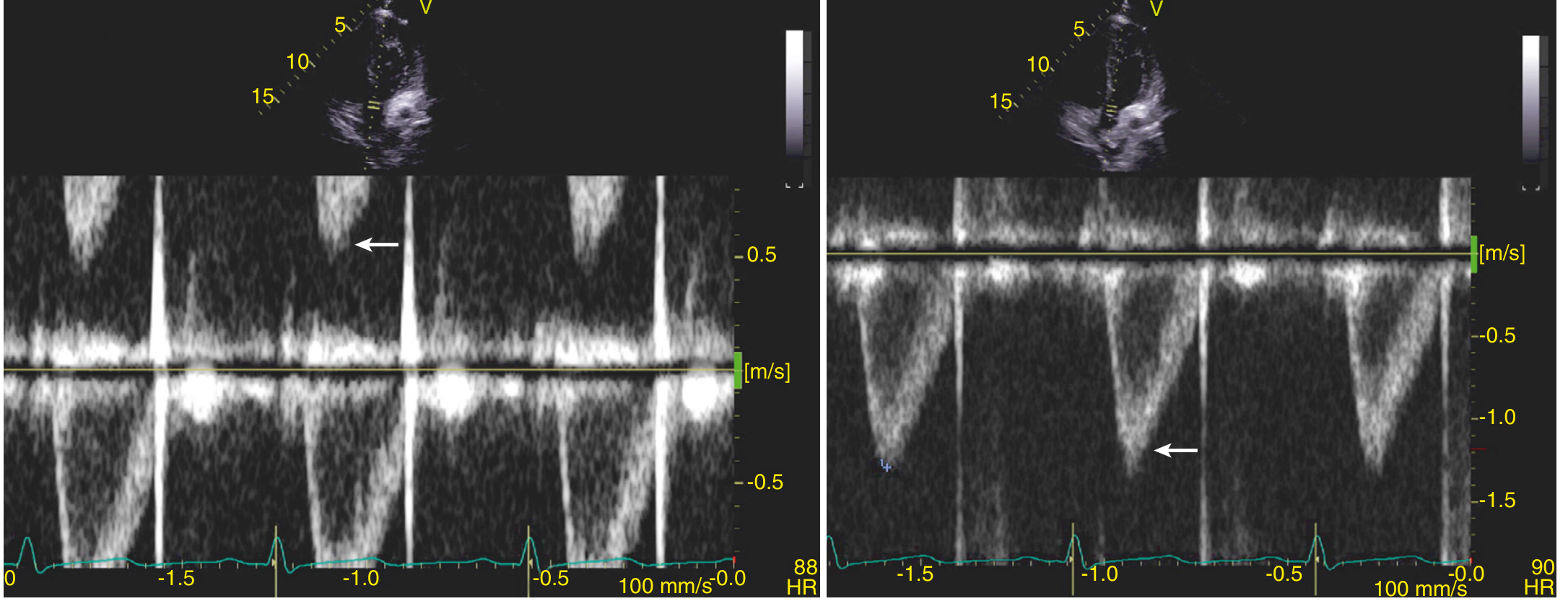
Spectral Analysis (Spectral Doppler)
The backscattered signal is analyzed by Fast Fourier Transform (FFT) to decompose the complex signal into its component frequencies. The resulting spectral display shows:
- X-axis: time
- Y-axis: velocity (m/s), with zero baseline in the center
- Above baseline: flow toward transducer
- Below baseline: flow away from transducer
- Gray scale brightness: signal amplitude (density of red blood cells at that velocity)
The spectral envelope = maximum velocity at each time point. The space under the envelope (when it is NOT solid/filled in) indicates laminar flow. A filled-in envelope indicates turbulent or disturbed flow with a wide range of velocities.
Continuous-Wave (CW) Doppler
- Uses two separate crystals - one continuously transmitting, one continuously receiving
- No range resolution: records ALL velocities along the entire beam length (range ambiguity)
- No upper velocity limit - can measure extremely high velocities (4-6 m/s in severe AS, MR, VSD)
- The envelope represents the maximum velocity anywhere along the beam
- Essential for quantifying stenotic and regurgitant lesions
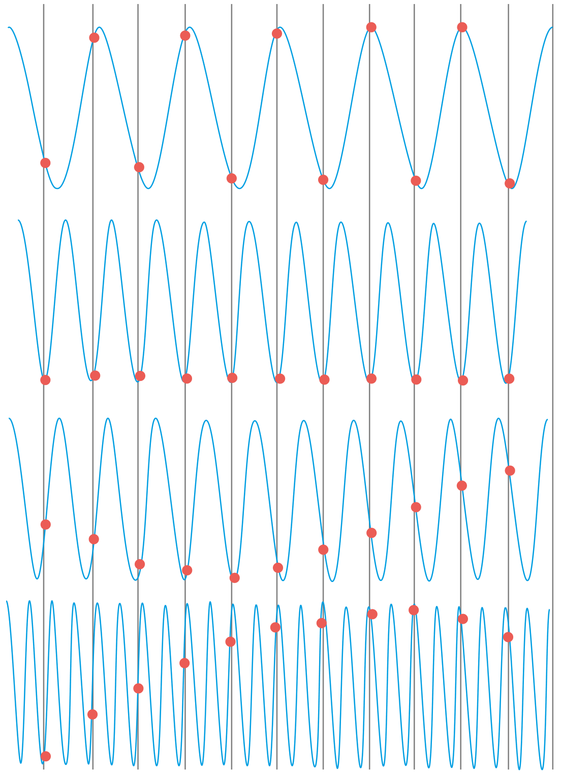
Pulsed-Wave (PW) Doppler
- Single crystal alternately transmits and receives
- Sample volume placed at a specific depth - allows range-specific velocity measurement
- Nyquist limit: the maximum velocity that can be unambiguously measured = PRF/2. If the Doppler shift exceeds this, aliasing occurs
- Nyquist limit typically 0.5-1.5 m/s - sufficient for normal intracardiac flows
- CANNOT measure high velocities without aliasing - use CW for those
Methods to resolve aliasing:
- Shift the baseline
- Use a lower-frequency transducer
- Increase PRF to maximum
- Use High-PRF Doppler (deliberate range ambiguity)
- Switch to CW Doppler
Aliasing on spectral display: the waveform appears "cut off" at the Nyquist limit and the remainder "wraps around" to the opposite channel.
Sampling principle (aliasing basis):
Color Flow Doppler (CFD)
Color Doppler is multi-gate pulsed Doppler applied simultaneously to hundreds of sample volumes across the 2D image:
- Red: flow toward transducer
- Blue: flow away from transducer
- Green/mosaic (variance): turbulence/high-velocity disturbed flow
- Velocity scale = color scale; aliasing appears as color reversal at the Nyquist limit
Color flow Doppler is used for:
- Detecting and mapping regurgitant jets
- Identifying stenotic flow jets
- Detecting shunts (ASD, VSD, PDA)
- Guiding sample volume placement for spectral Doppler
Color M-mode (CMM): Color Doppler superimposed on M-mode display; useful for timing of flow events.
Tissue Doppler Imaging (TDI)
TDI uses the same Doppler principles but with filters set to measure the low-velocity, high-amplitude signals from myocardial tissue rather than the high-velocity, low-amplitude signals from blood.
Mitral annular TDI:
- PW sample volume placed at medial (septal) or lateral MV annulus
- Measures e' (e-prime): early diastolic annular velocity
- Measures a': late diastolic annular velocity (atrial contribution)
- Measures s': systolic annular velocity (longitudinal systolic function)
Normal values (septal/lateral):
| Measure | Septal | Lateral |
|---|---|---|
| s' | ≥ 7 cm/s | ≥ 10 cm/s |
| e' | ≥ 8 cm/s | ≥ 10 cm/s |
E/e' ratio: Transmitral E velocity / annular e' velocity → estimates LV filling pressure
- E/e' < 8: normal LV filling pressure
- E/e' 8-14: indeterminate
- E/e' > 14: elevated LV filling pressure (mean PCWP > 15 mmHg)
PART 4: LEFT VENTRICULAR SYSTOLIC FUNCTION
Visual Assessment
The first step is always visual assessment of global and regional LV function. An experienced echocardiographer can categorize:
- Normal EF (≥ 55%)
- Mildly reduced EF (45-54%)
- Moderately reduced EF (35-44%)
- Severely reduced EF (< 35%)
Regional wall motion is assessed in 17 segments using the AHA model, scored as:
- Normal
- Hypokinetic (reduced motion and thickening)
- Akinetic (absent motion)
- Dyskinetic (paradoxical outward motion)
- Aneurysmal
Ejection Fraction by 2D (Biplane Simpson's Method of Disks)
The gold standard for LV EF measurement:
$$EF = \frac{EDV - ESV}{EDV} \times 100%$$
Simpson's method (Biplane method of disks):
- Trace endocardium in A4C and A2C views at end-diastole and end-systole
- LV is divided into a series of elliptical disks; total volume = sum of all disk volumes
- Avoids geometric assumptions that invalidate area-length method in regional disease
Normal LV volumes (indexed to BSA):
| Measure | Male | Female |
|---|---|---|
| LVEDVI | 34-74 mL/m² | 29-61 mL/m² |
| LVESVI | 11-31 mL/m² | 8-24 mL/m² |
| EF | 52-72% | 54-74% |
LV Linear Dimensions (from M-mode or 2D)
- LVIDd (end-diastolic diameter): Normal < 5.8 cm (M) / < 5.3 cm (F)
- LVIDs (end-systolic diameter): Normal < 3.9 cm - key follow-up parameter in chronic AR and MR
- IVSd and LVPWd: normal 0.6-1.0 cm; ≥ 1.3 cm = concentric hypertrophy (thresholds per ASE guidelines)
- Relative wall thickness (RWT) = (2 × PWd) / LVIDd: differentiates concentric from eccentric hypertrophy
Stroke Volume and Cardiac Output
The Doppler stroke volume is calculated from the LVOT:
$$SV = \pi (D/2)^2 \times VTI_{LVOT}$$
Where D = LVOT diameter (cm) and VTI = velocity-time integral of LVOT PW Doppler.
$$CO = SV \times HR$$
This is the cornerstone for:
- Continuity equation (valve area calculation)
- Valve regurgitation quantification
- Qp:Qs shunt calculation
- TAPSE and FAC for RV function
Global Longitudinal Strain (GLS)
Speckle tracking echocardiography (STE) tracks natural acoustic speckles in the myocardium frame-to-frame to derive myocardial deformation (strain):
$$\text{Strain} = \frac{\Delta L}{L_0} \times 100%$$
Where L₀ = original length, ΔL = change in length.
GLS = average peak longitudinal strain from all 17 segments. Normal GLS ≈ -20% to -22% (negative because the LV shortens longitudinally in systole).
Clinical value of GLS:
- More sensitive than EF for detecting subclinical LV dysfunction (e.g., in chemotherapy cardiotoxicity, pre-clinical HCM, hypertension)
- GLS > -16% (less negative) = significant dysfunction even with preserved EF
- Used in ASE/EACVI surveillance for cancer therapy-related cardiac dysfunction
- Braunwald notes: "Longitudinal systolic strain imaging has emerged as a more sensitive measure of LV function and predicts adverse clinical events, including mortality" in aortic stenosis
PART 5: LV DIASTOLIC FUNCTION
Diastolic dysfunction is common and clinically important. The 2016 ASE/EACVI guidelines use a 4-variable algorithm:
The Four Key Diastolic Parameters
1. Mitral inflow E/A ratio (PW Doppler, apical 4C, MV tips):
- E wave: early passive filling velocity
- A wave: late atrial kick velocity
- Normal E/A: 0.8-2.0; normal peak E: 50-100 cm/s
Diastolic filling patterns:
| Pattern | E/A | E-wave DT | Pathophysiology | LV filling pressure |
|---|---|---|---|---|
| Normal | 0.8-2.0 | 160-240 ms | Normal | Normal |
| Impaired relaxation (Grade I) | < 0.8 | > 240 ms | Slow LV relaxation | Normal or low |
| Pseudonormal (Grade II) | 0.8-2.0 | 160-200 ms | ↑ filling pressure normalizes pattern | Elevated |
| Restrictive (Grade III) | > 2 | < 160 ms | High atrial-LV pressure gradient | Markedly elevated |
Pseudonormal pattern is unmasked by:
- Valsalva maneuver: E/A drops to < 0.5 with true pseudonormalization
- TDI e' remains reduced despite normal E/A
2. Annular e' velocity (TDI):
- Medial e' < 7 cm/s OR lateral e' < 10 cm/s = diastolic dysfunction
- Relatively load-independent marker of relaxation
3. E/e' ratio: Integrates filling velocity with relaxation velocity → estimates PCWP
- Average E/e' (septal + lateral / 2) > 14 = elevated filling pressure
4. Peak TR velocity: Estimates PA systolic pressure via modified Bernoulli:
$$\Delta P = 4V^2$$
- PASP > 35 mmHg suggests elevated LA pressure
5. Left atrial volume index (LAVI):
- LA enlargement is a marker of chronic elevated filling pressure
- LAVI > 34 mL/m² indicates LA enlargement
ASE 2016 Diastolic Dysfunction Grading:
- Grade I (mild): Impaired relaxation; normal filling pressure (e' < lower limits; E/A < 0.8 + E < 50 cm/s)
- Grade II (moderate): Pseudonormal pattern; elevated filling pressure
- Grade III (severe): Restrictive physiology; markedly elevated filling pressure
PART 6: RIGHT HEART ASSESSMENT
RV Anatomy and Standard Measurements
The RV is a complex, crescent-shaped structure wrapping around the LV. Standard measurements:
- RV basal diameter (A4C): normal < 41 mm
- RV mid-cavity diameter: normal < 35 mm
- RVOT diameter (PLAX): normal < 33 mm
RV systolic function markers:
| Measure | Normal | Abnormal |
|---|---|---|
| TAPSE (tricuspid annular plane systolic excursion) | ≥ 17 mm | < 17 mm |
| RV FAC (fractional area change) | ≥ 35% | < 35% |
| TDI s' (RV free wall) | ≥ 9.5 cm/s | < 9.5 cm/s |
| RV GLS | ≥ -20% | < -20% |
Pulmonary Artery Pressure Estimation
PA systolic pressure (PASP):
$$PASP = 4 \times V_{TR}^2 + RAP$$
Where V_TR = peak TR velocity and RAP = estimated RA pressure from IVC.
IVC-based RA pressure estimation:
- IVC ≤ 2.1 cm + collapses > 50% with sniff → RAP = 3 mmHg
- IVC > 2.1 cm + collapses < 50% → RAP = 15 mmHg
- Intermediate → RAP = 8 mmHg
Pulmonary vascular resistance (PVR) - Abbas formula:
$$PVR = \frac{TR_{Vmax}}{RVOT_{VTI}} \times 10$$
- PVR < 2 Wood units = normal
Pulmonary Artery Acceleration Time (PAAT)
PW Doppler in the PA. Normally, flow accelerates to peak velocity by mid-systole (PAAT > 100 ms). With elevated pulmonary vascular resistance:
- PAAT < 100 ms suggests pulmonary hypertension
- PAAT < 70 ms indicates severe PHT
- Mid-systolic notching of the PA flow profile is pathognomonic of severe pulmonary arterial hypertension
PART 7: VALVULAR HEART DISEASE
Aortic Stenosis (AS) - The Most Quantified Valve Lesion
As Braunwald's Heart Disease states: "Doppler echocardiography allows measurement of indices to determine the severity of AS, including peak transvalvular jet velocity...mean transvalvular pressure gradient, and aortic valve area (AVA) (calculated using the continuity equation)"
Severity classification (ASE/AHA/ACC):
| Parameter | Mild | Moderate | Severe |
|---|---|---|---|
| Peak jet velocity | 2.0-2.9 m/s | 3.0-3.9 m/s | ≥ 4.0 m/s |
| Mean gradient | < 20 mmHg | 20-39 mmHg | ≥ 40 mmHg |
| AVA | > 1.5 cm² | 1.0-1.5 cm² | < 1.0 cm² |
| Indexed AVA | > 0.85 cm²/m² | 0.60-0.85 | < 0.60 cm²/m² |
Modified Bernoulli equation:
$$\Delta P = 4V^2$$
(Simplified - assumes proximal velocity is negligible)
Full Bernoulli: ΔP = 4(V₂² - V₁²) - used when LVOT velocity > 1.5 m/s (avoids overestimation)
Continuity equation for AVA:
$$AVA = \frac{CSA_{LVOT} \times VTI_{LVOT}}{VTI_{AV}}$$
$$= \frac{\pi(D_{LVOT}/2)^2 \times VTI_{LVOT}}{VTI_{AV}}$$
Or using peak velocities: AVA = (LVOT area × V_LVOT) / V_AV
Dimensionless index (DVI): V_LVOT / V_AV = proxy for AVA without needing LVOT diameter measurement. DVI < 0.25 = severe AS.
Low-flow, low-gradient AS: When EF is reduced (<50%) AND mean gradient < 40 mmHg AND AVA < 1.0 cm². Use dobutamine stress echo to differentiate true severe AS (AVA remains <1.0 cm² as flow increases) from pseudo-severe AS (AVA normalizes with increased flow).
Mitral Stenosis (MS)
Pressure half-time (PHT) method for MVA:
$$MVA = \frac{220}{T_{1/2}}$$
The pressure half-time is the time for the peak transmitral gradient to fall by half; measured from the deceleration slope of the E-wave.
- T₁/₂ > 150 ms = significant MS
- MVA < 1.5 cm² = significant MS; < 1.0 cm² = severe MS
Wilkins score for balloon commissurotomy suitability (each criterion 1-4):
- Leaflet mobility
- Leaflet thickening
- Subvalvular thickening
- Calcification Total score < 8 = good candidate for PMC
Planimetry of MVA: In PSAX at MV leaflet tips (direct measurement); superior to PHT in:
- After commissurotomy (PHT overestimates MVA post-PMC)
- With significant AR (PHT overestimates MVA)
- With reduced LV compliance
Mitral Regurgitation (MR) - Quantification
Qualitative: Color jet area / LA area (crude, affected by many factors)
Semi-quantitative:
- Vena contracta width (VC): narrowest width of the color jet at origin
- VC ≥ 7 mm = severe MR
- Jet density on CW Doppler: dense, triangular signal = severe MR
- Pulmonary vein flow: systolic flow reversal = severe MR
Quantitative - PISA (Proximal Isovelocity Surface Area) method:
The most accurate non-invasive method:
$$ERO = \frac{2\pi r^2 \times V_{aliasing}}{V_{MR}}$$
$$R_{Vol} = ERO \times VTI_{MR}$$
Where:
- r = PISA radius (measured at aliasing velocity V_aliasing)
- V_MR = peak MR jet velocity
Severe primary MR criteria (ASE):
| Parameter | Severe |
|---|---|
| ERO | ≥ 0.40 cm² |
| Regurgitant volume | ≥ 60 mL |
| Regurgitant fraction | ≥ 50% |
| Vena contracta | ≥ 7 mm |
Aortic Regurgitation (AR)
Severity assessment:
- Color Doppler jet width in LVOT: severe AR when jet width ≥ 65% of LVOT diameter
- Pressure half-time: PHT < 200 ms = severe AR (rapid pressure equalization)
- Holodiastolic flow reversal in descending aorta: severe AR
- Vena contracta: ≥ 6 mm = severe AR
- EROA/RVol by PISA
Braunwald on AR follow-up: "Sequential evaluations of LV end-systolic dimension in patients with chronic valve regurgitation" - LVIDs is the key trigger for intervention (≥ 50 mm per AHA/ACC guidelines).
PART 8: ADVANCED TOPICS
Stress Echocardiography
Principle: Regional wall motion abnormalities (RWMA) appear during ischemia before ECG changes or symptoms (ischemic cascade). Normal myocardium increases in contractility during stress.
Modalities:
- Exercise echo: treadmill (peak exercise) or bicycle (continuous imaging during exercise)
- Dobutamine stress echo (DSE): dobutamine infusion from 5-40 mcg/kg/min + atropine if needed; target HR = 85% max predicted (220-age × 0.85)
- Pharmacological vasodilators: adenosine/regadenoson (nuclear preferred; occasionally echo)
- Dipyridamole echo: European standard
Interpretation of DSE for ischemia:
- Normal: all segments hyperkinetic at peak stress
- Ischemia: new RWMA at any stage (hypokinesia, akinesia, dyskinesia)
- Viable hibernating myocardium: wall motion improves at low-dose dobutamine (biphasic response)
- Fixed scar: no change at any dose
Braunwald emphasizes: "Exercise echocardiography" as a key approach combining functional anatomy with provokable ischemia assessment.
Sensitivity ~85%, specificity ~80-85% for detecting obstructive CAD.
Transesophageal Echocardiography (TEE)
TEE positions the transducer in the esophagus and stomach, eliminating the chest wall as a barrier. Because the esophagus lies posterior to the heart:
- Posterior structures (LA, LAA, pulmonary veins, MV, interatrial septum) are seen with exceptional clarity
- Anterior structures (aortic arch, LVOT, prosthetic aortic valve) are slightly deeper
Standard TEE views by probe position and angle:
| Position | Omniplane Angle | View |
|---|---|---|
| Mid-esophageal | 0-20° | 4-chamber |
| Mid-esophageal | 60-75° | 2-chamber (LA, LV) |
| Mid-esophageal | 120-135° | Long-axis |
| Mid-esophageal | 30-60° | AV short-axis |
| Upper esophageal | 0° | Aortic arch |
| Transgastric | 0° | SAX LV (papillary level) |
| Deep transgastric | 0° | True apical (LV outflow) |
Unique clinical indications for TEE:
- Cardiac source of embolism: LA thrombus, LAA thrombus (sensitivity ~98% vs. ~<60% for TTE), PFO, ASD
- Infective endocarditis: Vegetations, perivalvular abscess (TEE sensitivity 90-95% vs. 50-60% TTE)
- Aortic dissection: Type A/B; sensitivity 97-99%
- Intraoperative monitoring: Cardiac surgery guidance
- Structural interventions: Real-time guidance for TAVR, MitraClip, LAA occlusion, ASD closure
- Prosthetic valve dysfunction: Pannus, thrombus, paravalvular leak
- Poor TTE windows
Contrast Echocardiography
Indications for LV opacification (LVO) contrast:
- Two or more contiguous LV segments not adequately visualized on non-contrast study
- Critical for accurate EF quantification in poor acoustic windows
Agents: Microbubble contrast agents (e.g., Definity, Optison, SonoVue) with lipid or albumin shells filled with perfluorocarbon gas. Microbubbles resonate at the ultrasound frequency, dramatically enhancing backscatter.
Techniques:
- Harmonic imaging: receive at 2f₀ - myocardium suppressed, contrast enhanced
- Low mechanical index (MI): preserves microbubbles; MI < 0.3 for perfusion imaging
- Destruction-replenishment (high MI flash followed by low MI): maps myocardial perfusion
Myocardial perfusion imaging (MPI) with contrast: Can detect microvascular obstruction and distinguish viable from non-viable myocardium.
Intracardiac Echocardiography (ICE)
A catheter-based ultrasound transducer introduced via femoral vein into the right heart. Uses phased array or rotational elements at 5-10 MHz.
Applications:
- Guiding transseptal puncture (real-time visualization of needle/catheter crossing fossa ovalis)
- Guidance of: PFO closure, ASD device closure, AF ablation, TAVR, LAAC
- Increasingly replacing TEE for structural interventions (avoids general anesthesia)
Cardiac Output and Hemodynamic Assessment
Fick principle vs. Doppler CO: Doppler is accurate with parallel alignment and careful measurement.
Non-invasive hemodynamics by echo:
| Parameter | Method | Normal |
|---|---|---|
| LVEDP | E/e' > 15; MV B-bump on M-mode | < 12 mmHg |
| PCWP | E/e' ratio; pulmonary vein flow | < 15 mmHg |
| PASP | 4 × V_TR² + RAP | < 35 mmHg |
| PADP | 4 × V_ED-PR² + RAP (from end-diastolic PR jet) | < 12 mmHg |
| PVR | V_TR/VTI_RVOT × 10 | < 2 WU |
Pericardial Disease
Pericardial effusion assessment:
- Trivial: < 5 mm posterior to LV
- Small: 5-10 mm
- Moderate: 10-20 mm
- Large: > 20 mm
- Cardiac tamponade: Effusion + hemodynamic compromise. Echo signs:
- RA collapse in late diastole/early systole (sensitive, >90%)
- RV diastolic collapse (specific)
- Plethoric IVC (> 2.1 cm, < 50% collapse)
- Exaggerated respiratory variation in MV/TV inflow velocities (> 25%/> 40%)
- "Swinging heart"
Constrictive pericarditis vs. restrictive cardiomyopathy:
| Feature | Constrictive | Restrictive |
|---|---|---|
| Septal bounce | Present | Absent |
| Respiratory variation in E | > 25% | < 10% |
| TDI e' | Normal or elevated (annulus paradox ≥ 9 cm/s) | Reduced (< 7 cm/s) |
| Hepatic vein flow | Expiratory reversals | Inspiratory reversals |
Cardiomyopathies
Hypertrophic Cardiomyopathy (HCM):
- Diagnosis: Wall thickness ≥ 15 mm (in any segment) in absence of other cause; ≥ 13 mm with family history or positive genetics
- Distribution: ASH (asymmetric septal hypertrophy) most common; basal, midventricular, apical variants
- LVOTO: Systolic anterior motion (SAM) of MV → dynamic LVOT obstruction
- Gradient > 30 mmHg at rest or provocation = significant obstruction
- Provocation: Valsalva maneuver increases obstruction
- Assessment: Measure resting and provoked LVOT gradient with CW Doppler; characteristic "dagger-shaped" CW envelope
- SAM: the anterior MV leaflet is dragged into the LVOT during systole by Venturi forces and drag forces
Dilated Cardiomyopathy (DCM):
- LV dilation + reduced EF; wall motion globally impaired
- Distinguish ischemic (territorial RWMA) from non-ischemic (global, diffuse)
- LV sphericity (sphericity index): Round LV suggests more severe DCM
- Functional MR common: dilated annulus + papillary muscle displacement
Amyloidosis:
- Biventricular hypertrophy + granular sparkling texture (older imaging)
- Diastolic dysfunction (restrictive pattern)
- Low EF despite preserved wall thickness ("MOGE-S" deception: thick walls but low voltage on ECG)
- GLS pattern: apical sparing (basal worse than apical strain) - highly specific for cardiac amyloidosis
- Low MAPSE (mitral annular plane systolic excursion)
Congenital Heart Disease (Brief Overview)
Atrial Septal Defect (ASD):
- Right heart enlargement pattern (RV/RA dilation, volume overload septal motion)
- Subcostal view for IAS anatomy; TEE for complete characterization
- 2D + color Doppler identifies defect and flow; size guides closure decision
- Qp:Qs > 1.5:1 generally indicates hemodynamically significant shunt
VSD:
- Color jet across IVS; CW gradient estimates RV systolic pressure
- Restrictive VSD: high velocity (>4 m/s), small RV enlargement
- Non-restrictive: equalization of ventricular pressures
PART 9: BIOEFFECTS AND SAFETY
All diagnostic ultrasound exams must follow the ALARA principle (As Low As Reasonably Achievable). Two bioeffect indices are displayed on all modern ultrasound machines:
-
Thermal Index (TI): Estimated temperature rise (°C) at a specific tissue location. TI < 1.0 for routine cardiac imaging; TI < 0.7 in fetal imaging.
- TIS = soft tissue; TIB = bone; TIC = cranial bone
-
Mechanical Index (MI): Indicator of the likelihood of cavitation. MI = P_neg (MPa) / √f (MHz). Normal diagnostic: MI < 1.9. Contrast imaging requires MI < 0.3 to avoid microbubble destruction.
Three bioeffect categories:
- Thermal: heating from absorption of mechanical energy. Rate = 2αI/ρCm. Clinically negligible at diagnostic levels.
- Cavitation: gas bubble creation/vibration. Resonance frequency F₀ = 3260/R₀ (microns). Not demonstrated at diagnostic levels without contrast agents.
- Other: micro streaming, torque forces - only at much higher intensities than diagnostic.
PART 10: KEY CLINICAL DECISION-MAKING
When to Use Which Echo Technique
| Clinical Question | Best Modality |
|---|---|
| LV EF | 2D biplane Simpson's (3D if available) |
| LV mass | M-mode (linear) or 2D area-length |
| Valve stenosis severity | CW Doppler + continuity equation |
| Regurgitation severity | PISA + VCW + PV flow |
| Diastolic function | E/A + TDI e' + E/e' + LAVI |
| LA thrombus | TEE (>TTE) |
| Endocarditis - valve complications | TEE |
| RVSP | TR jet CW + IVC |
| SAM in HCM | CW from apex + M-mode |
| Guidance of structural interventions | 3D TEE / ICE |
| Subclinical LV dysfunction | GLS (speckle tracking) |
Braunwald's Indications for Echocardiography (Class I)
From Braunwald's Heart Disease (Block 11):
- Evaluation and follow-up of known or suspected valvular heart disease
- Assessment of LV function when clinical decision depends on result
- Suspected myocardial disease (cardiomyopathy, myocarditis)
- Suspected cardiac source of embolism
- Suspected aortic disease
- Suspected pericardial disease
- Evaluation of suspected congenital heart disease
- Re-evaluation when clinical status changes
Summary Reference Table: Normal Echo Values
| Parameter | Normal Value |
|---|---|
| LV EF | ≥ 52% (M) / ≥ 54% (F) |
| LVIDd | < 5.8 cm (M) / < 5.3 cm (F) |
| IVSd / LVPWd | 0.6-1.0 cm (normal) / ≥ 1.3 cm (hypertrophy) |
| LA volume index | < 34 mL/m² |
| Aortic root (sinus) | ≤ 2.1 cm/m² |
| E/A (MV inflow) | 0.8-2.0 |
| TDI e' (septal) | ≥ 8 cm/s |
| TDI e' (lateral) | ≥ 10 cm/s |
| E/e' average | < 14 |
| GLS | -20% to -22% |
| TAPSE | ≥ 17 mm |
| RV basal diameter | < 41 mm |
| PASP | < 35 mmHg |
| IVC (normal) | ≤ 2.1 cm, > 50% collapse |
| AVA (normal) | ≥ 2.0 cm² |
| MVA (normal) | 4-6 cm² |
References:
- Otto CM, Schwaegler RG, Freeman RV. Textbook of Clinical Echocardiography, 6e (ISBN 9780323882088)
- Braunwald's Heart Disease: A Textbook of Cardiovascular Medicine, 12e (ISBN 9780323722193), Chapters on Echocardiography (Blocks 9, 10, 11)
- ASE/EACVI 2015 Recommendations for Cardiac Chamber Quantification
- ASE/EACVI 2016 Recommendations for the Evaluation of Left Ventricular Diastolic Function
This is a shared conversation. Sign in to Orris to start your own chat.