
How to set contrast in mri brain filming
MRI brain filming contrast settings typically refer to window/level (W/L) settings used when displaying or printing MRI images. Here's a quick overview:
- T1-weighted: Window ~300-400, Level ~150-200 (bright white matter, gray GM/CSF contrast)
- T2-weighted: Window ~400-600, Level ~200-300 (bright CSF, good gray/white differentiation)
- FLAIR: Similar to T2 but CSF suppressed - window ~300-500, level ~150-250
- DWI/ADC: Narrower windows to highlight diffusion abnormalities
These are starting points - final settings depend on scanner, field strength, and clinical goal.
Searching sources...
Reading File
Searching the Web
MRI brain filming window level contrast settings radiology
Finding Sources
Finding Sources
Reading Web Page
https://www.mdpi.com/2813-9038/2/3/11
Reading File
Here is a thorough guide on setting contrast (window/level) for MRI brain filming:
MRI Brain Filming: Setting Contrast (Window/Level)
Core Concept: Window Width (WW) and Window Level (WL)
Contrast in MRI filming is controlled by two parameters:
| Parameter | What it controls | Effect |
|---|---|---|
| Window Width (WW) | The range of signal intensities displayed | Narrow WW = higher contrast, fewer gray shades; Wide WW = lower contrast, more gray shades |
| Window Level (WL) | The center/brightness point of that range | Higher WL = darker image (focused on brighter structures); Lower WL = brighter image |
All signal intensities below the window floor appear black; all above the ceiling appear white. Only values within the window are shown in grayscale.
Recommended Settings by MRI Sequence
| Sequence | Window Width (WW) | Window Level (WL) | Purpose |
|---|---|---|---|
| T1-weighted | 300-400 | 150-200 | Shows anatomy clearly - white matter bright, gray matter intermediate |
| T2-weighted | 400-600 | 200-300 | CSF is bright (white), white matter dark, pathology stands out |
| FLAIR | 300-500 | 150-250 | Like T2 but with CSF suppressed; periventricular lesions highlighted |
| DWI | 200-400 | 100-200 | Restricted diffusion (strokes, abscess) appears bright |
| ADC map | 800-1000 | 400-600 | Opposite of DWI - restricted areas appear dark |
| T1 + Gadolinium (contrast) | 300-400 | 150-200 | Enhancing lesions (tumors, inflammation) stand out as bright |
| SWI / GRE | 200-400 | 100-200 | Narrow to highlight microhemorrhages (appear very dark) |
Note: These are starting ranges. Actual values depend on your MRI scanner, field strength (1.5T vs 3T), and the specific pulse sequence parameters used.
Step-by-Step Approach
-
Start with scanner defaults - most PACS/filming workstations auto-apply a default window for each sequence type. Review these first.
-
Adjust WL for brightness - if the brain looks too dark, lower the WL; if too washed out/bright, raise it.
-
Adjust WW for contrast - if lesions blend in with surrounding tissue, narrow the WW to increase contrast. If too much noise/artifacts are visible, widen the WW slightly.
-
Use sequence-specific optimization:
- For T2/FLAIR: prioritize showing CSF-tissue boundaries clearly
- For DWI: narrow WW to make acute strokes "pop"
- For T1+Gad: ensure enhancing lesions are distinctly brighter than non-enhancing tissue
-
Apply the "narrower WW = better lesion conspicuity" rule - research in musculoskeletal MRI confirms that a narrower window width relative to the window level significantly improves visibility of pathological signal changes (e.g., edema).
-
Check bone/skull edges - if assessing for skull base or calvarium lesions, you may need to widen the window temporarily.
Practical Tips
- Most radiologists do not use a single fixed setting - they scroll through windows dynamically during reading, adjusting interactively on PACS.
- Right-click drag on most PACS systems adjusts W/L in real time (horizontal drag = width, vertical drag = level).
- Pre-programmed presets by body region are available on most scanners and filmers (e.g., "brain soft tissue," "posterior fossa," "orbit").
- When filming for print (hard copy), use settings that preserve visible gray-white differentiation without over-brightening - typically a medium WW and WL centered around the brain parenchyma signal.
- For contrast-enhanced studies (gadolinium), some centers slightly narrow the WW compared to the pre-contrast T1 to make enhancement more conspicuous.
As noted in Neuroanatomy through Clinical Cases 3rd Edition, window and level "determine the conversion between the calculated density values and the gray scale used for display" - the same principle applies to MRI signal intensities as to CT Hounsfield units, though MRI values are arbitrary (scanner-dependent) rather than standardized like HU.
Mri brain intracranilangio planing with image
MRI brain intracranial angiography (MRA - Magnetic Resonance Angiography) planning involves positioning slabs to cover the circle of Willis and major intracranial vessels. Key sequences include TOF (Time of Flight) and PC (Phase Contrast) MRA.
Searching sources...
Reading File
Searching the Web
MRI brain intracranial MRA planning TOF angiography positioning protocol images
Finding Sources
Reading Web Page
https://mrimaster.com/plan-mra-brain
Loading Image
Finding Sources
Loading Image
Reading File
Searching the Web
MRA brain TOF planning slab circle of willis axial positioning diagram
Loading Image
Loading Image
Loading Image
Here is a complete guide to MRI Brain Intracranial Angiography (MRA) planning:
MRI Brain Intracranial Angiography (MRA) - Planning Guide
What is Brain MRA?
MRA (Magnetic Resonance Angiography) of the brain visualizes the intracranial arteries - primarily the Circle of Willis and its branches - without ionizing radiation. The standard method is 3D Time-of-Flight (TOF) MRA, which requires no contrast injection in most cases.
Indications
- Intracranial aneurysm (screening and follow-up)
- Arteriovenous malformation (AVM)
- Cerebral arterial stenosis / occlusion
- Stroke work-up
- Vasculitis
- Moyamoya disease
- Post-treatment follow-up (clipping, coiling)
MRA Vessels Visualized (Circle of Willis Anatomy)
The TOF MRA beautifully shows all major intracranial vessels:
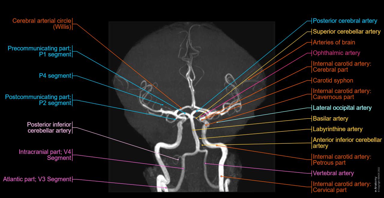
Full intracranial vessel anatomy on TOF MRA - showing ICA segments, basilar artery, vertebral arteries, cerebellar arteries, and Circle of Willis
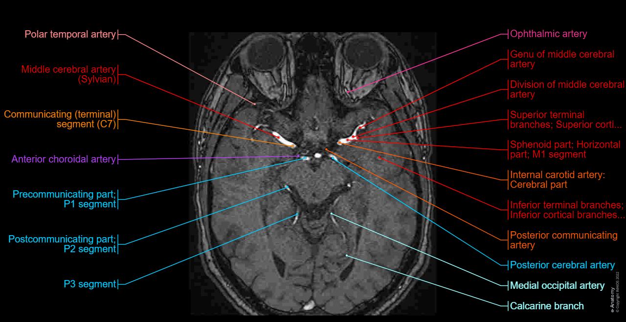
Axial TOF source image showing MCA (M1), ICA, PCA, P-comm, and anterior choroidal artery
Step-by-Step Planning Protocol
Step 1 - Patient Positioning
- Position: Head-first supine
- Place head in the head coil, immobilize with foam pads/cushions
- Center the laser landmark over the glabella (bridge of nose)
- Give earplugs for noise; instruct patient to remain still
Step 2 - Run 3-Plane Localizer
- Quick 3-plane scout (~25 seconds, T1 low resolution)
- Provides axial, sagittal, and coronal reference images for planning all sequences
Step 3 - Plan the 3D TOF MRA Slab
This is the most important step:
| Plane | How to Plan |
|---|---|
| Sagittal view | Angle the axial 3D block parallel to the genu and splenium of the corpus callosum |
| Coronal view | Ensure the block is perpendicular to the 3rd ventricle and brainstem (to correct for head tilt) |
| Coverage | From 1 cm above the corpus callosum down to the foramen magnum (to include basilar tip and posterior fossa) |
Key rule: Avoid excessive angulation - the slab should be as straight (axial) as possible to avoid flow-related signal loss and artifacts.
Step 4 - Add Saturation Band
- Place a Superior Saturation (SAT) band on top of the axial block
- This suppresses venous signal (superior sagittal sinus, cortical veins) so only arterial flow is shown
- Without the SAT band, veins will also enhance and contaminate the MIP images
Step 5 - MIP Reconstruction
- After acquisition, the raw data is post-processed using Maximum Intensity Projection (MIP)
- MIPs are generated in multiple angles (every 15-20°, full 360° rotation) to show vessel anatomy from all directions
- Targeted sub-volume MIPs can be made for specific regions (e.g., isolated left MCA territory)
Recommended Protocol Parameters (3D TOF MRA)
| Parameter | Value |
|---|---|
| Sequence | 3D GRE / FLASH (Siemens), SPGR (GE), FFE (Philips) |
| TR | 25-35 ms |
| TE | 3.5-7 ms (shortest possible) |
| Flip Angle | 15-25° |
| Slice Thickness | 0.5-1.0 mm (isotropic preferred) |
| Slab Thickness | 60-80 mm (covers full Circle of Willis) |
| FOV | 200-230 mm |
| Matrix | 512 x 512 (or 320-384 minimum) |
| Orientation | Axial |
| SAT band | Superior (venous suppression) |
| MT pulse | Magnetization Transfer ON (improves vessel-to-background contrast) |
| Scan time | 5-8 minutes (single slab), 8-12 min (multi-slab) |
At 3T: Higher SNR allows thinner slices (0.5 mm isotropic) and better small vessel detail. At 1.5T: Slightly thicker slices (0.7-1.0 mm) are standard.
Single Slab vs. Multiple Overlapping Slabs (MOTSA)
| Method | Use |
|---|---|
| Single 3D slab | Faster, good for Circle of Willis only |
| MOTSA (Multiple Overlapping Thin-Slab Acquisition) | Better coverage, reduced saturation effects in large vessels; used when examining full intracranial tree |
Also Included in a Brain MRA Study
Most protocols add routine brain sequences alongside the MRA:
- T2 TSE Axial - parallel to corpus callosum genu/splenium, full brain coverage
- FLAIR Axial - same angulation as T2
- DWI - for acute stroke assessment
- T1 axial - for anatomical reference and pre/post contrast comparison if needed
What to Look for on the Final MRA
- Circle of Willis completeness (complete in only ~40% of people) - Grainger & Allison's Diagnostic Radiology
- Aneurysm (focal outpouching, usually at vessel bifurcations)
- Stenosis or occlusion (signal dropout, "rat's tail" appearance in dissection)
- AVM (tangle of vessels with early venous filling)
- Asymmetry of vessel caliber
Tutorial Video
For a step-by-step visual walkthrough on Siemens 1.5T/3T, this tutorial covers the exact planning steps:
This is a shared conversation. Sign in to Orris to start your own chat.