
Define proteins and explain structural organization with diagrams examples and bonds between them add note on denaturation of proteins
protein structure levels primary secondary tertiary quaternary diagram
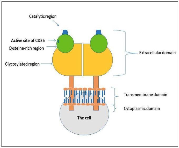
This medical illustration depicts the quaternary protein structure of CD26 (Dipeptidylpeptidase IV), presented as a homodimeric type II transmembrane glycoprotein. The diagram illustrates two identical subunits arranged symmetrically across the plasma membrane. Each subunit is divided into three primary functional domains: the extracellular domain, the transmembrane domain, and the cytoplasmic domain. The large extracellular domain is further subdivided into a catalytic region at the distal end, an active site (represented as a green sphere), a cysteine-rich region, and a glycosylated region (represented by yellow structures). The transmembrane domain is shown as an alpha-helical structure traversing the lipid bilayer, represented by a schematic of blue phospholipids with orange spheres. The cytoplasmic domain is depicted as a grey semi-circle extending into the cell interior. This schematic provides a fundamental educational overview of the molecular architecture of CD26, highlighting the orientation and localization of domains responsible for its enzymatic and non-enzymatic signaling functions.

Summary : This figure presents a structured overview of the three levels of disease prevention and health promotion (primary, secondary, tertiary) as applied to the management of malnutrition, frailty, and sarcopenia in patients with cirrhosis. It details aims, assessment strategies, and actions for each prevention level, and highlights the use of diagnostic and management toolboxes. flowchart/table hybrid: # Structure : • The figure is organized as a multi-row, multi-column table with flowchart elements. • Columns represent: Primary prevention, Secondary prevention, Tertiary prevention, and a final box for "Prevent the occurrence of undesirable health outcomes". • Rows represent: Aim, Assessment, Action. • Overlapping horizontal bars for "Diagnostic toolbox" and "Management toolbox" span relevant sections. # Columns (Prevention Levels) : • Primary prevention: Focuses on preventing development and delaying onset. • Secondary prevention: Focuses on early diagnosis, prompt initiation of treatment, and slowing progression. • Tertiary prevention: Focuses on rehabilitation and reversal. • Final box: "Prevent the occurrence of undesirable health outcomes". # Rows (Content Areas) : ## Aim : • Primary: Prevent development, delay onset. • Secondary: Early diagnosis, prompt initiation of treatment, slow progression. • Tertiary: Rehabilitate, reverse. ## Assessment : • Primary: Malnutrition screening, assessment of muscle dysfunction. • Secondary: Evaluate for etiologic risk factors, explore dietary preferences and barriers to exercise. • Tertiary: Reassess for progression of malnutrition, frailty, and/or sarcopenia despite primary and secondary preventative efforts. ## Action : • Primary: Educate patients and caregivers, encourage positive health behaviors, empower patients with specific skills. • Secondary: Apply management toolbox, co-management with registered dietitian and certified exercise physiologist/physical therapist if available. • Tertiary: Refer to registered dietitian, certified exercise physiologist/physical therapist, and/or health behavior specialist for co-management; consider center-based rehabilitation, intensive nutritional supplementation. # Toolboxes : • Diagnostic toolbox: Spans assessment row for primary and secondary prevention. • Management toolbox: Spans action row for secondary and tertiary prevention. # Layout : • Table format with horizontal flow from left (primary) to right (tertiary), culminating in prevention of undesirable outcomes. • Colour-coded sections: orange for primary/secondary, green for tertiary. # Analysis : • The figure visually organizes the progression from prevention to management in cirrhosis care, emphasizing a stepwise approach. • Each prevention level builds on the previous, with increasing intervention intensity. • The use of toolboxes highlights the integration of diagnostic and management strategies across levels. • The final outcome box underscores the goal of preventing undesirable health outcomes through tailored interventions at each stage.
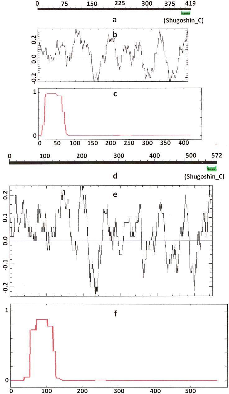
This image is a comparative bioinformatics diagram illustrating the secondary structure and biochemical properties of shugoshin proteins: A. thaliana SGO2 (top panels a-c) and SGO1 (bottom panels d-f). Panel (a) shows the primary sequence of SGO2 (419 amino acids) with a highlighted C-terminal 'Shugoshin_C' functional domain. Panel (d) shows SGO1 (572 amino acids) with a similar C-terminal domain. Panels (b) and (e) present line graphs of the electrostatic charge distribution across the protein length, oscillating between approximately -0.2 and 0.2, used to identify localized positive charge peaks. Panels (c) and (f) provide a COILS program prediction of the probability (0 to 1 on the y-axis) of forming alpha-helical secondary structures. In both proteins, a high-probability alpha-helical region is observed near the N-terminus, which corresponds with functional conservation despite low primary sequence similarity. This visualization is used in molecular genetics to compare mitotic (SGO2) and meiotic (SGO1) protein variants and their structural conservation in centromere localization.
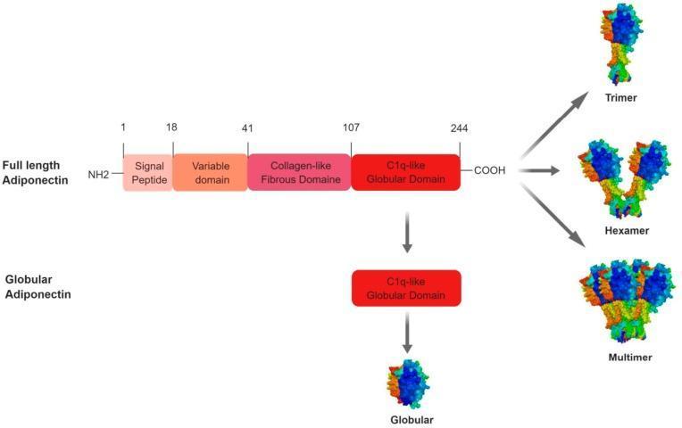
This pathophysiology diagram illustrates the primary structural domains and oligomeric forms of human adiponectin. The 'Full length Adiponectin' (244 amino acids) is depicted as a linear protein sequence originating from the NH2-terminus. It comprises four distinct domains labeled with their starting amino acid positions: the Signal Peptide (aa 1), Variable domain (aa 18), Collagen-like Fibrous Domain (aa 41), and the C1q-like Globular Domain (aa 107), terminating at the COOH-terminus (aa 244). Below this, 'Globular Adiponectin' is shown as a standalone C1q-like domain, representing the proteolytic short form of the protein. The right side of the diagram presents three-dimensional molecular models demonstrating the protein's quaternary structure: a Trimer (low molecular weight), a Hexamer (medium molecular weight), and a complex Multimer (high molecular weight). The diagram serves as an educational resource to explain the post-translational polymerization and domain organization essential for adiponectin's biological activity in metabolic and endocrine signaling.
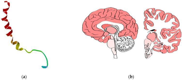
This composite educational graphic illustrates the structural and anatomical context of Neuropeptide Y (NPY), a key orexigenic peptide. (a) A 3D molecular ribbon diagram shows the secondary structure of the 36-amino acid NPY peptide. It features a prominent C-terminal alpha-helix (red-yellow) and a flexible N-terminal polyproline-like fold, forming the characteristic 'PP-fold' tertiary structure. A color gradient from red to blue highlights residues along the sequence length. (b) A sagittal cross-section and (c) a coronal section of the human brain provide anatomical landmarks for NPY expression. Visible structures include the cerebral cortex with detailed gyri and sulci, the thalamus, hypothalamus (the primary site of orexigenic regulation), cerebellum, and brainstem (pons and medulla). The diagram maps the high expression of NPY within these central nervous system regions. The visual serves to bridge the molecular biology of the NPY gene and its product with clinical neuroanatomy, relevant to pharmacological studies on antipsychotic-induced weight gain and metabolic regulation.
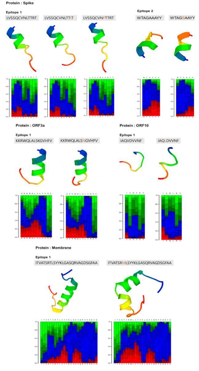
Educational structural bioinformatics plot illustrating the predicted 3D conformations of SARS-CoV-2 epitopes (Spike, ORF3a, ORF10, and Membrane proteins) following amino acid substitutions. Each panel consists of a PEP-FOLD3 ribbon diagram showing secondary structure alongside a corresponding local structure prediction profile bar graph. The ribbon models utilize color-coded gradients (blue to red) to represent the N-to-C terminal progression and conformational states. Below each model, heatmaps indicate the probability of local structural motifs: red indicates helical (alpha-helix) regions, green represents extended (beta-sheet) conformations, and blue denotes coil/random structures. The visualization demonstrates how specific mutations, such as T175M in the Membrane protein or V30L in ORF10, influence the tertiary folding and structural flexibility of B-cell and T-cell candidate antigens. This comparison is critical for evaluating how viral variants may impact epitope recognition and vaccine efficacy.
alpha helix beta sheet secondary structure protein
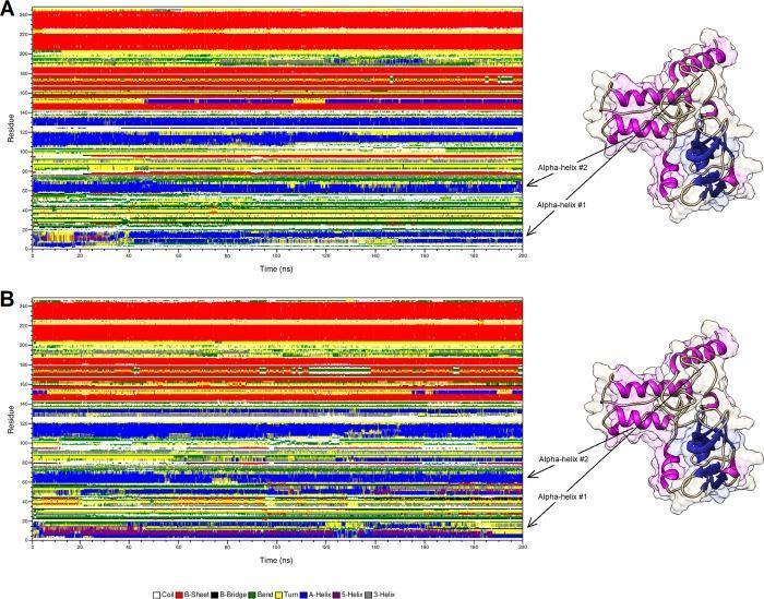
This bioinformatics infographic displays a secondary structure comparison between wild-type Brain-Derived Neurotrophic Factor (BDNF) (A) and its V66M variant (B) using Molecular Dynamics (MD) simulations. The central components are two time-evolution heatmaps (residue number vs. time in nanoseconds, 0-200 ns) showing the stability and transitions of protein motifs. A standardized color key identifies structural elements: white for coils, red for beta-sheets, black for beta-bridges, green for bends, yellow for turns, blue for alpha-helices, purple for 5-helices, and gray for 3-helices. To the right of each heatmap, a 3D ribbon-and-surface protein model highlights specific alpha-helices (Alpha-helix #1 and #2) for spatial orientation. Comparison reveals temporal shifts in secondary structure stability, particularly in the N-terminus and pre-domain regions of the V66M variant. The red beta-sheet regions show increased density in the V66M variant compared to the wild-type, while alpha-helical regions exhibit altered temporal patterns. This visualization illustrates how single-point mutations like V66M can impact protein folding and essential molecular motions related to neurodevelopmental pathways.
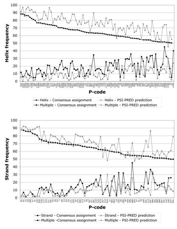
This Comparison Chart consists of two line graphs analyzing protein secondary structure assignments and predictions across various 'P-codes' (representing hydrophobic cluster species). The top graph displays 'Helix frequency' (alpha-helices), and the bottom graph displays 'Strand frequency' (beta-strands). Each graph compares two primary datasets: a 'Consensus assignment' derived from multiple experimental methods and a 'PSI-PRED prediction' computational model. Additionally, both graphs track 'Multiple' assignments, where clusters are associated with more than one secondary structure. The educational focus is on evaluating the accuracy of the PSI-PRED algorithm in structural biology. Key trends show that PSI-PRED consistently over-predicts regular secondary structures (helices and strands) compared to experimental consensus, while under-representing 'multiple' or ambiguous assignments. Visually, the consensus lines show a steady downward trend in frequency as the P-code increases, whereas the PSI-PRED predictions exhibit higher variability and smoother fluctuations. This illustrates the potential for algorithmic over-estimation of regular secondary structures at the expense of structural complexity in protein bioinformatics.
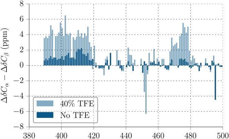
This Comparison Chart displays experimental secondary structure propensities of Axin-1 (residues 390-500) derived from Nuclear Magnetic Resonance (NMR) chemical shift measurements. The y-axis represents the difference in chemical shifts (ΔδCα - ΔδCβ) in parts per million (ppm), while the x-axis lists residue numbers. The graph compares two conditions: with 40% Trifluoroethanol (TFE), a known alpha-helix stabilizer (light blue bars), and without TFE (dark blue bars). Consecutive positive values indicate alpha-helical propensity, most prominently observed in the regions of residues 390-420 and 470-480. In the presence of 40% TFE, these helical propensities are significantly enhanced, reaching shifts above 4 ppm. Conversely, negative values indicate beta-sheet propensity, visible around residues 450 and 500. The data illustrates how TFE modulates the transient secondary structures of this intrinsically disordered protein region, highlighting key binding sites for GSK3β and β-catenin. This diagram is utilized in molecular biology and biochemistry to analyze protein folding and conformational dynamics.
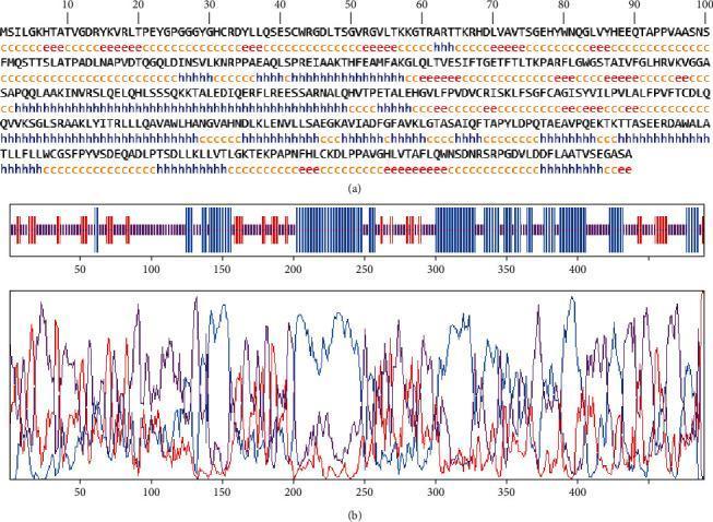
This figure presents the results of a bioinformatic analysis of the secondary structure of the ROP29 protein, a protein relevant in medical microbiology and infectious disease research. Panel (a) shows the primary amino acid sequence with GOR4 secondary structure predictions mapped directly beneath each residue. Predictions are represented by letter codes: 'h' (blue) for alpha-helix, 'e' (red) for extended strand (beta-sheet), 'c' (orange) for random coil, and 't' (purple) for turn. This linear map allows for the identification of specific structural domains along the 489-residue sequence. Panel (b) consists of two graphical plots. The upper plot in (b) is a color-coded barcode representation of structural propensity along the sequence length. The lower plot in (b) is a line graph displaying the statistical probability or propensity scores of secondary structures (blue and red lines) across the amino acid positions. These tools are used in vaccine development and proteomics to predict epitope accessibility and protein folding characteristics. The analysis highlights that the protein is predominantly composed of random coils (49.69%) and alpha-helices (36.81%).
Proteins: Definition, Structural Organization, Bonds, and Denaturation
Definition of Proteins
- Structural support - collagen, keratin
- Enzymatic catalysis - amylase, pepsin, DNA polymerase
- Transport - hemoglobin (O2), albumin (lipids, drugs)
- Immune defense - immunoglobulins (antibodies)
- Signaling - insulin, growth hormone, receptors
- Contractile/motor - actin, myosin
- Storage - ferritin (iron), casein (milk protein)
"Proteins are composed of amino acids that are joined together by peptide bonds in a linear sequence, and then folded into a unique three-dimensional shape that determines function." - Biochemistry, Lippincott Illustrated Reviews, 8th ed.
Building Block: The Amino Acid and Peptide Bond
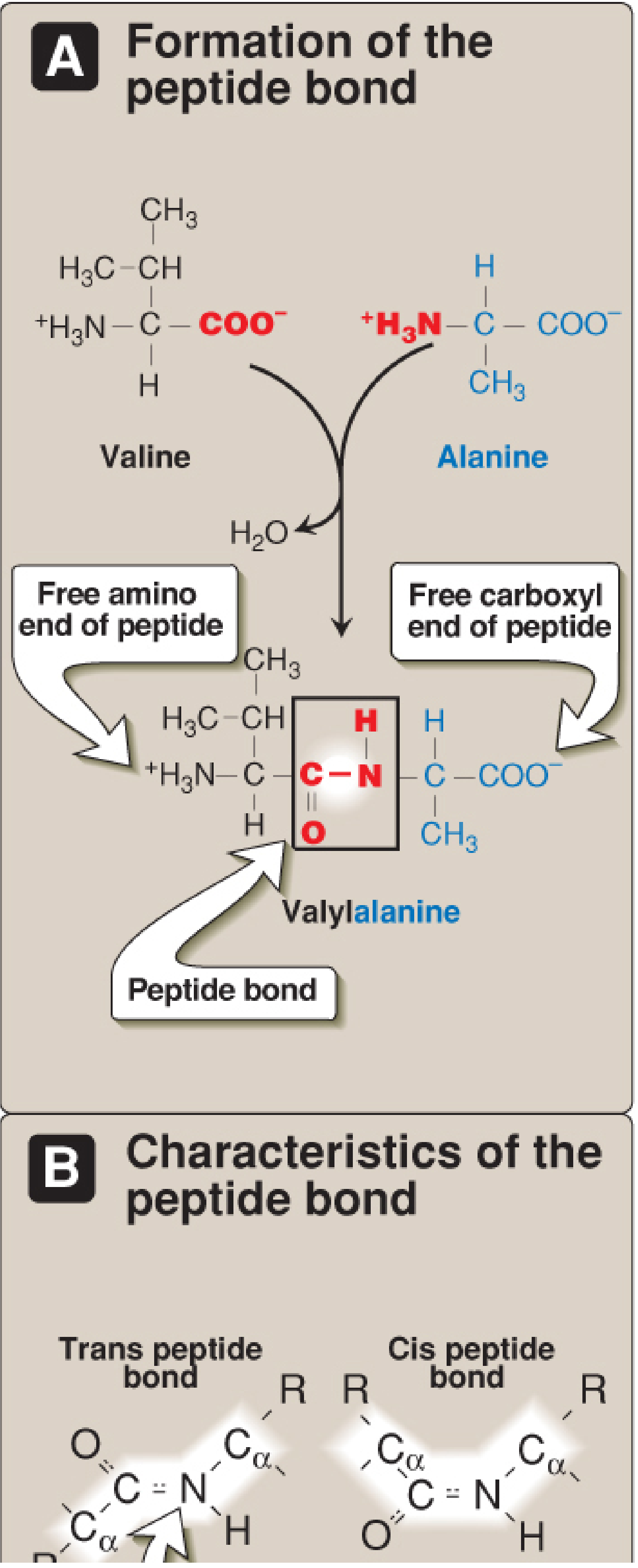
- Has partial double-bond character - rigid and planar, shorter than a single bond
- Almost always in the trans configuration (R groups on opposite sides)
- Uncharged (-C=O and -NH groups) but polar - participate in hydrogen bonds
- Resistant to mild heat and urea, but broken by strong acid/base at elevated temperature
- Convention: N-terminal (free amino end) written to the LEFT; C-terminal to the RIGHT
Four Levels of Protein Structure
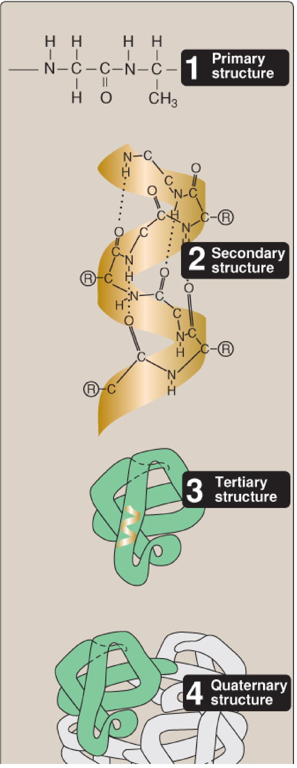
1. PRIMARY STRUCTURE
- Written from N-terminus (left) to C-terminus (right)
- 50+ amino acids = polypeptide / protein; shorter = peptide
- Genetic mutations can change even a single amino acid and cause disease (e.g., sickle cell anemia: glutamate → valine at position 6 of β-globin)
- The primary structure dictates all higher levels of structure
2. SECONDARY STRUCTURE
a) Alpha-Helix (α-Helix)
- A right-handed spiral (clockwise when viewed from top)
- Stabilized by intramolecular hydrogen bonds between the C=O of one peptide bond and the N-H of the peptide bond 4 residues ahead
- Each turn contains 3.6 amino acid residues
- R groups point outward from the helical axis
- Proline disrupts the α-helix (its cyclic structure prevents the proper dihedral angles)
- Examples: α-keratin (hair, nails, skin), myoglobin (highly helical)
b) Beta-Sheet (β-Sheet / β-Pleated Sheet)
- Formed by extended polypeptide strands lying side by side
- All peptide bond C=O and N-H groups are involved in inter-strand hydrogen bonds
- Successive α-carbons are slightly above/below the plane, giving a "pleated" appearance
- Strands can be parallel (same N→C direction) or antiparallel (opposite N→C direction)
- Strands are often shown as broad arrows in structural diagrams
- Examples: Silk fibroin (nearly all β-sheet), immunoglobulin domains, β-barrel pores
c) Beta-Bends (β-Turns / Hairpin Loops)
- Reverse the direction of the polypeptide chain by ~180°
- Allow the chain to fold back on itself
- Often connect adjacent antiparallel β-strands
- Stabilized by hydrogen bonds and frequently contain proline or glycine
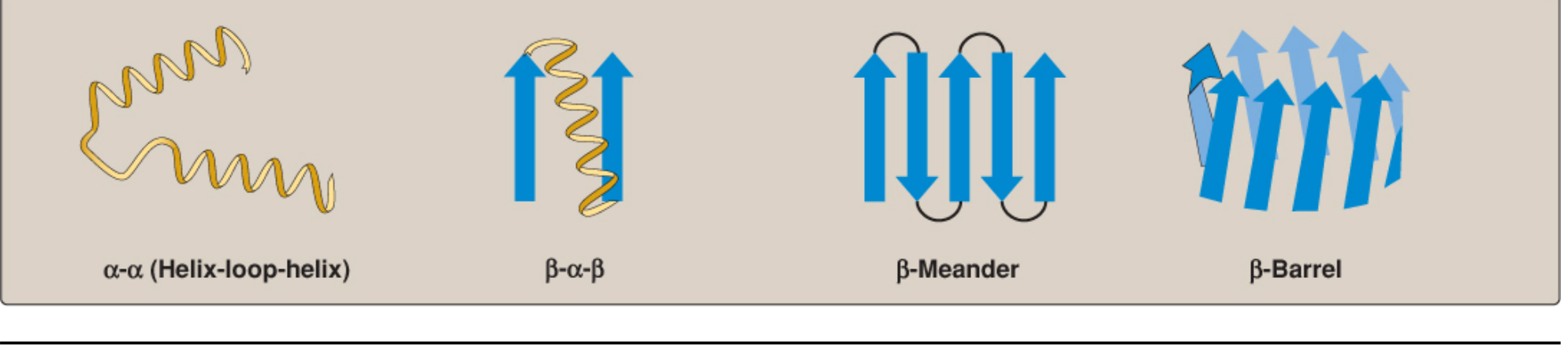
| Motif | Description |
|---|---|
| α-α (Helix-loop-helix) | Two α-helices connected by a loop; seen in DNA-binding transcription factors |
| β-α-β | β-strand, α-helix, β-strand unit; common in nucleotide-binding proteins |
| β-Meander | Sequential antiparallel β-strands connected by tight loops |
| β-Barrel | Multiple β-strands rolled into a barrel shape; seen in porin channels |
3. TERTIARY STRUCTURE
- Compact, globular shape with a densely packed hydrophobic core
- Hydrophobic R groups buried inside; hydrophilic R groups on the surface
- Chains >200 aa typically fold into multiple domains (semi-independent folding units)
Four Types of Bonds/Interactions Stabilizing Tertiary Structure:
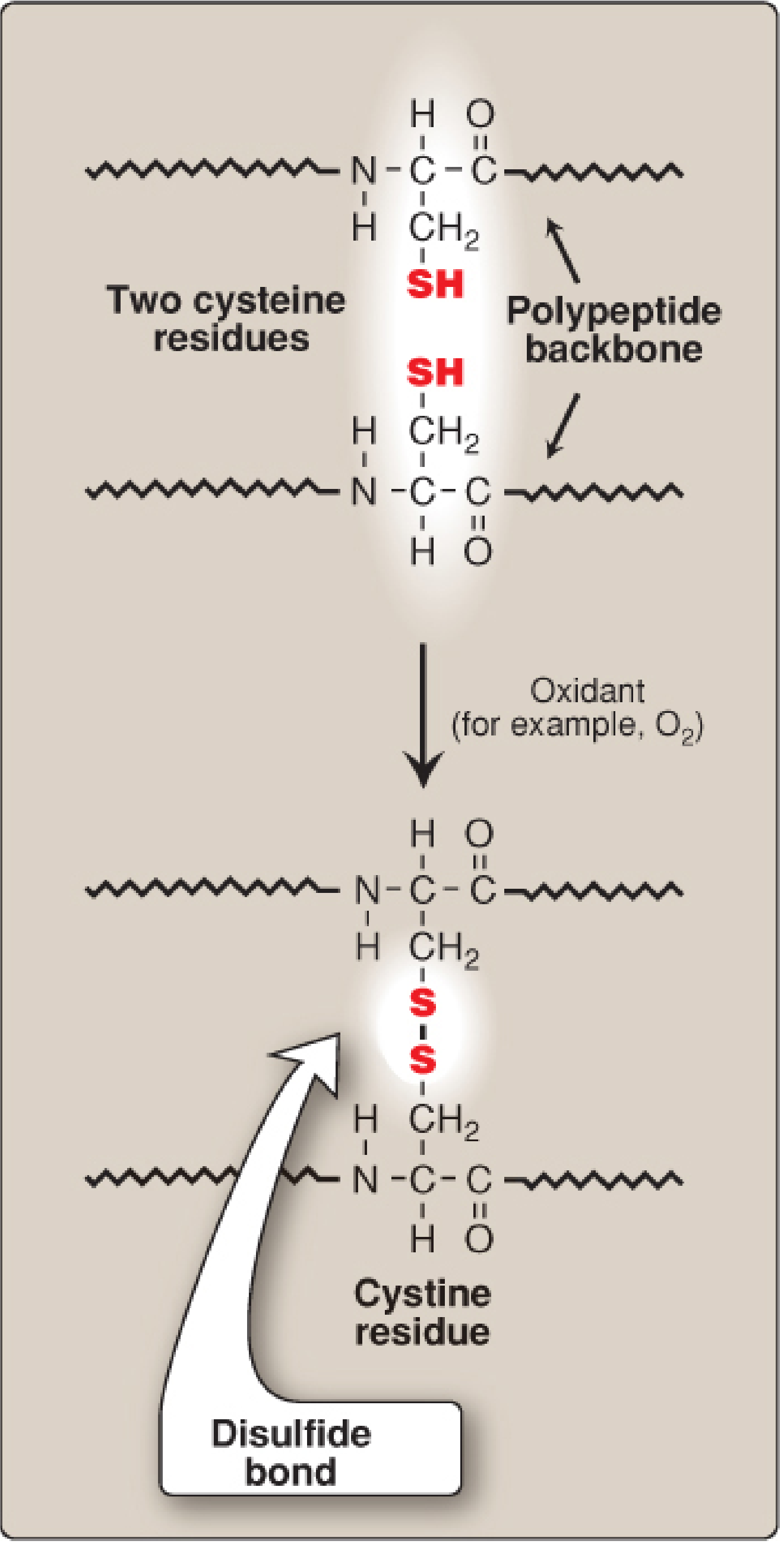
- Formed by oxidation of two -SH groups from two cysteine residues → S-S bond, producing a cystine residue
- Can be within a chain (intrachain) or between chains (interchain)
- Common in extracellular/secreted proteins (e.g., immunoglobulins, insulin)
- Contributes rigidity and prevents denaturation in the extracellular environment
- Nonpolar R groups (leucine, isoleucine, valine, phenylalanine) cluster in the interior, away from water
- Thermodynamically driven - burying hydrophobic groups releases organized water molecules (increase in entropy)
- The dominant force driving protein folding in aqueous environments
- Between polar side chains (e.g., -OH of serine/threonine with -C=O of backbone or other side chains)
- Also between surface groups and surrounding water - increases solubility
- Individually weak, but collectively very significant due to large number
- Between oppositely charged R groups: e.g., negatively charged -COO⁻ of aspartate/glutamate ↔ positively charged -NH₃⁺ of lysine/arginine
- Often on the protein surface; disrupted by extreme pH changes
| Bond Type | Strength | Example |
|---|---|---|
| Peptide bond | Strong (covalent) | Backbone linkage |
| Disulfide bond | Strong (covalent) | Cys-Cys in immunoglobulins |
| Hydrogen bond | Weak (non-covalent) | α-helix, β-sheet, Ser-OH to backbone |
| Hydrophobic interaction | Moderate (non-covalent) | Leu, Ile core packing |
| Ionic/salt bridge | Weak (non-covalent) | Asp-COO⁻ ... Lys-NH₃⁺ |
| Van der Waals | Very weak | Close-packed nonpolar atoms |
- Myoglobin - highly helical, single domain, oxygen-storage protein in muscle
- Lysozyme - mix of α and β, antibacterial enzyme in tears/saliva
- Ribonuclease A - stabilized by 4 disulfide bonds
4. QUATERNARY STRUCTURE
- Subunits may be identical (homomeric) or different (heteromeric)
- Held together by non-covalent interactions (hydrogen bonds, hydrophobic interactions, ionic bonds); sometimes also by disulfide bonds
- Subunits may act independently or cooperatively
| Arrangement | Term | Example |
|---|---|---|
| 2 subunits | Dimer | HIV protease (homodimer) |
| 3 subunits | Trimer | Collagen (heterotrimer: 2α1 + 1α2) |
| 4 subunits | Tetramer | Hemoglobin (2α + 2β subunits) |
Note on Denaturation of Proteins
Definition
"Denaturation results in the unfolding and disorganization of a protein's secondary and tertiary structures without the hydrolysis of peptide bonds." - Lippincott Biochemistry, 8th ed.
Agents That Cause Denaturation
| Agent | Mechanism |
|---|---|
| Heat | Disrupts H-bonds, hydrophobic interactions; causes aggregation |
| Extreme pH (acid/base) | Alters ionization of R groups; disrupts ionic bonds and H-bonds |
| Urea / guanidinium chloride | Compete with intra-protein H-bonds; unfold structure |
| Organic solvents (ethanol, acetone) | Disrupt hydrophobic interactions and H-bonds |
| Detergents (SDS) | Bind nonpolar regions; unfold hydrophobic core |
| Heavy metals (Pb²⁺, Hg²⁺) | React with -SH groups; disrupt disulfide bonds |
| Reducing agents (DTT, β-mercaptoethanol) | Break disulfide bonds |
| Nonenzymatic glycation | Glucose binds amino groups, cross-links form, protein aggregates (seen in diabetes - HbA1c formation) |
What Happens During Denaturation
- Hydrophobic groups originally buried in the core become exposed
- The protein loses its specific 3D shape (native conformation)
- Biological activity is lost (enzyme cannot catalyze, receptor cannot bind)
- Protein often becomes insoluble and precipitates from solution (e.g., cooked egg white)
Reversibility
- Under ideal conditions, removal of the denaturing agent can allow the protein to refold (renaturation) - the classic example is ribonuclease A, which was fully renatured after urea + β-mercaptoethanol removal (Anfinsen experiment, 1961)
- In most real-world cases, denaturation is irreversible - permanently disordered aggregates form
Chaperones and Denaturation Prevention
- Hsp70 - binds hydrophobic regions of unfolded/nascent chains, keeps them unfolded until synthesis is complete
- Hsp60 (GroEL in bacteria) - cage-like structure where unfolded protein enters, folds, and is released (ATP-dependent)
- After denaturation, most proteins cannot be rescued by chaperones and remain permanently unfolded
Clinical Relevance
- Protein-losing nephropathy/enteropathy - loss of native serum proteins
- Prion diseases - misfolded proteins (PrP^Sc) that resist normal denaturation and cause normal PrP^C to misfold; irreversible
- Diabetes mellitus - sustained hyperglycemia causes nonenzymatic glycation of proteins (collagen, hemoglobin), forming advanced glycation end products (AGEs) that cross-link and aggregate, damaging tissue
- Sterilization - autoclaving kills microbes by denaturing their proteins (121°C steam under pressure)
- Urea (8M) in labs - fully unfolds proteins for analysis
Summary Table: Four Levels of Protein Structure
| Level | Definition | Stabilizing Bond | Example |
|---|---|---|---|
| Primary | Amino acid sequence | Peptide bond (covalent) | Sickle cell Hb (Val→Glu) |
| Secondary | Local helix/sheet folding | Hydrogen bonds (backbone) | α-Keratin (hair), β-silk |
| Tertiary | Overall 3D shape | H-bonds, hydrophobic, ionic, disulfide | Myoglobin, lysozyme |
| Quaternary | Multi-subunit assembly | Non-covalent + disulfide | Hemoglobin, collagen |
Urine cycle Reaction energetics regulation difference between cps1 and cps2 metabolic disorders