Primary structure of proteins. The specificity, properties of peptide bond. Secondary and tertiary structure of proteins and bonds which stabilize them

Reading File

Finding Sources

Searching Images

protein primary secondary tertiary structure diagram

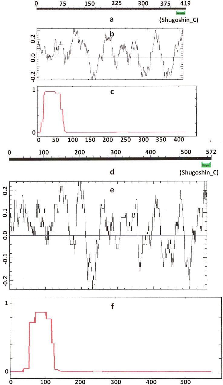
This image is a comparative bioinformatics diagram illustrating the secondary structure and biochemical properties of shugoshin proteins: A. thaliana SGO2 (top panels a-c) and SGO1 (bottom panels d-f). Panel (a) shows the primary sequence of SGO2 (419 amino acids) with a highlighted C-terminal 'Shugoshin_C' functional domain. Panel (d) shows SGO1 (572 amino acids) with a similar C-terminal domain. Panels (b) and (e) present line graphs of the electrostatic charge distribution across the protein length, oscillating between approximately -0.2 and 0.2, used to identify localized positive charge peaks. Panels (c) and (f) provide a COILS program prediction of the probability (0 to 1 on the y-axis) of forming alpha-helical secondary structures. In both proteins, a high-probability alpha-helical region is observed near the N-terminus, which corresponds with functional conservation despite low primary sequence similarity. This visualization is used in molecular genetics to compare mitotic (SGO2) and meiotic (SGO1) protein variants and their structural conservation in centromere localization.

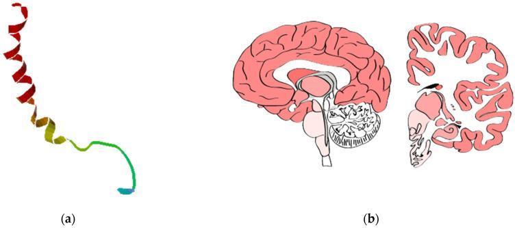
This composite educational graphic illustrates the structural and anatomical context of Neuropeptide Y (NPY), a key orexigenic peptide. (a) A 3D molecular ribbon diagram shows the secondary structure of the 36-amino acid NPY peptide. It features a prominent C-terminal alpha-helix (red-yellow) and a flexible N-terminal polyproline-like fold, forming the characteristic 'PP-fold' tertiary structure. A color gradient from red to blue highlights residues along the sequence length. (b) A sagittal cross-section and (c) a coronal section of the human brain provide anatomical landmarks for NPY expression. Visible structures include the cerebral cortex with detailed gyri and sulci, the thalamus, hypothalamus (the primary site of orexigenic regulation), cerebellum, and brainstem (pons and medulla). The diagram maps the high expression of NPY within these central nervous system regions. The visual serves to bridge the molecular biology of the NPY gene and its product with clinical neuroanatomy, relevant to pharmacological studies on antipsychotic-induced weight gain and metabolic regulation.

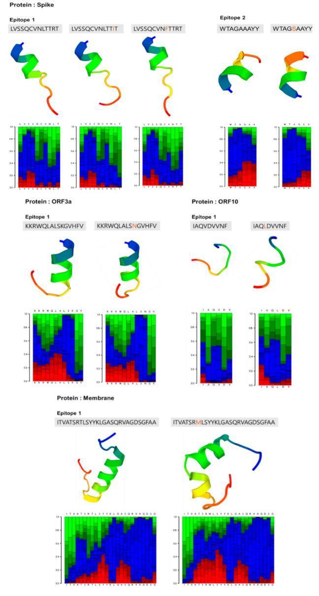
Educational structural bioinformatics plot illustrating the predicted 3D conformations of SARS-CoV-2 epitopes (Spike, ORF3a, ORF10, and Membrane proteins) following amino acid substitutions. Each panel consists of a PEP-FOLD3 ribbon diagram showing secondary structure alongside a corresponding local structure prediction profile bar graph. The ribbon models utilize color-coded gradients (blue to red) to represent the N-to-C terminal progression and conformational states. Below each model, heatmaps indicate the probability of local structural motifs: red indicates helical (alpha-helix) regions, green represents extended (beta-sheet) conformations, and blue denotes coil/random structures. The visualization demonstrates how specific mutations, such as T175M in the Membrane protein or V30L in ORF10, influence the tertiary folding and structural flexibility of B-cell and T-cell candidate antigens. This comparison is critical for evaluating how viral variants may impact epitope recognition and vaccine efficacy.

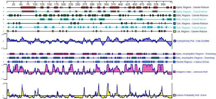
This bioinformatics diagram displays a comprehensive secondary structure and physicochemical property analysis of the human GPC3 (Glypican-3) protein sequence, spanning approximately 580 amino acids. The top section visualizes predicted secondary structural elements (Alpha-helices, Beta-sheets, Turns, and Coils) comparing the Garnier-Robson and Chou-Fasman algorithms. Below the structural predictions, several line graphs and plots represent protein characteristics: a Kyte-Doolittle Hydrophilicity Plot identifying hydrophobic and hydrophilic domains; Eisenberg plots for alpha and beta amphipathic regions; a Karplus-Schulz Flexible Regions plot; a Jameson-Wolf Antigenic Index highlighting potential epitope regions; and an Emini Surface Probability Plot predicting amino acid exposure. The data is aligned along a single horizontal axis representing the amino acid residue number, facilitating the identification of C-terminal regions rich in beta-turns and irregular coils. This visual serves as an educational tool for protein engineering and vaccine design, specifically for identifying antigenic subunits in oncological research.

Reading File

Finding Sources

Reading File

Finding Sources

Searching Images

peptide bond partial double bond character planar resonance

Multi-planar postoperative Magnetic Resonance Imaging (MRI) of the paranasal sinuses and skull base following partial resection of a primary Ewing’s sarcoma of the sphenoid sinus. The figure displays five views: (A) Axial T1-weighted image (T1WI), (B) Axial T2-weighted image (T2WI), (C) Axial T1WI with contrast enhancement, (D) Coronal T1WI with contrast enhancement, and (E) Sagittal T1WI with contrast enhancement. The images visualize a residual soft tissue mass (indicated by a black arrow in panel C) centered in the right sphenoid sinus cavity. The residual tumor demonstrates irregular borders and extends into the right orbital apex and the lateral aspect/tip of the right orbit. Post-contrast images (C, D, and E) show heterogeneous enhancement of the mass, suggesting residual vascularized tumor tissue. Visible surgical changes include partial resection of the sphenoid and ethmoid sinus walls. The images provide clinical evidence for assessing surgical margins and planning adjuvant therapy for aggressive small round cell tumors in the head and neck region.

Multi-planar abdominal computed tomography (CT) scan with intravenous contrast demonstrating a complication following laparoscopic sleeve gastrectomy. The image is divided into four panels: (A) coronal view, (B) sagittal oblique projection, and (C/D) axial views. The primary finding is the partial intrasplenic displacement of an 8.5 Fr double-pigtail stent, originally placed to manage a gastric staple-line leak. In panel B, a red arrow highlights the distal tip of the radiopaque stent migrating along the vessel axis toward the splenic parenchyma. In axial panel D, a red arrow indicates a focal pocket of subcapsular air within the spleen, a pathognomonic sign confirming the malposition of the drain and violation of the splenic capsule. The imaging illustrates a rare iatrogenic complication of endoscopic internal drainage where the stent migrates from the perigastric collection into adjacent solid organ structures. This case is relevant for surgical and radiological education regarding the monitoring of endoscopic stents and the identification of post-operative anatomical displacement.

This diagnostic image displays functional Magnetic Resonance Imaging (fMRI) results superimposed on standard axial, sagittal, and coronal anatomical scans. The figure illustrates multi-planar views of several neural clusters exhibiting significant functional connectivity changes (FDR-corrected p < 0.05) between placebo and probiotic intervention groups during an emotional attention task (EAT). Each panel presents a primary large axial slice (labeled with z-coordinates such as z=15, z=21, z=30) accompanied by smaller sagittal and coronal localized views to characterize the 3D spatial extent of the clusters. Bright orange-to-yellow clusters highlight specific areas of altered activity, including regions in the frontal cortex, parietal lobes, and occipital areas (as indicated by the peak MNI coordinates x, y, z provided below each set). Double-headed arrows indicate functional connectivity relationships or comparisons between specific clusters. This visual data is used in neuroscience and psychiatric research to study the gut-brain axis, demonstrating how probiotic interventions can modulate connectivity within predefined brain networks and the Brainnetome atlas (BNA).

Finding Sources

Reading File

Loading Image

I now have all the content and images needed for a comprehensive, well-illustrated answer. Let me compose it.

Protein Structure: Primary, Secondary, and Tertiary

Overview

Proteins are organized into four hierarchical levels of structure: primary, secondary, tertiary, and quaternary. Each level builds on the one below it.

Four levels of protein structure - primary (linear chain), secondary (alpha helix), tertiary (3D fold), quaternary (multi-subunit)

Figure 2.1 - Four hierarchies of protein structure (Lippincott's Illustrated Reviews: Biochemistry)

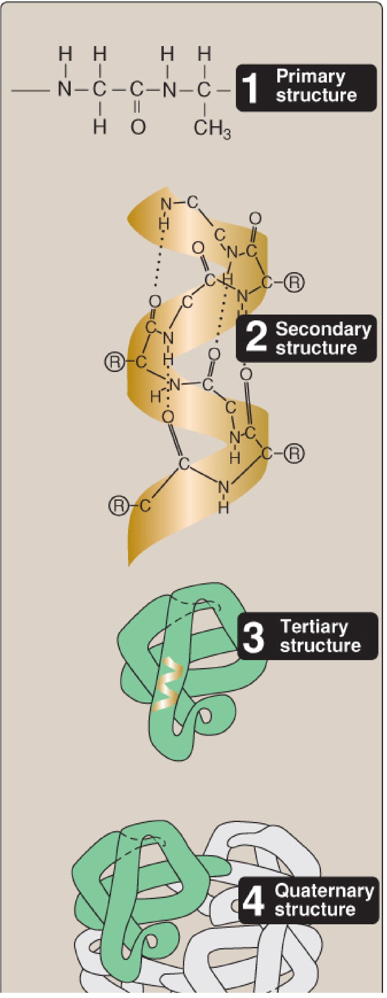
I. Primary Structure

The primary structure is the linear sequence of amino acids in a polypeptide chain, read from the N-terminal (free amino) end to the C-terminal (free carboxyl) end. It is the simplest and most fundamental level of protein organization.

The sequence is encoded directly in the gene.
Genetic mutations that alter the primary sequence can cause disease by disrupting protein folding and function (e.g., the single amino acid substitution in sickle cell hemoglobin: Glu → Val at position 6 of the β-chain).
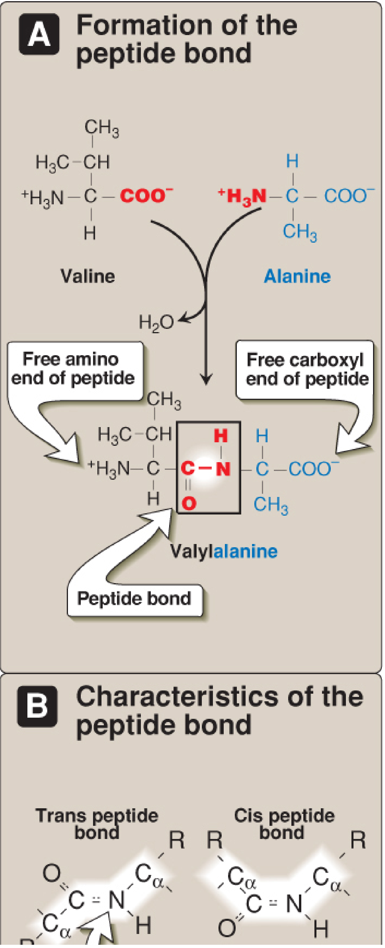
Each component amino acid in the chain is called a residue, because it represents the portion remaining after water is lost during peptide bond formation.
A chain of 50 or more amino acids joined by peptide bonds is called a polypeptide.

"The linear sequence of amino acids in a protein is the primary structure of the protein. Many genetic diseases result in proteins with abnormal amino acid sequences, causing improper folding and loss or impairment of normal function." - Biochemistry, 8th ed., Lippincott Illustrated Reviews, p. 50

II. The Peptide Bond

A. Formation

A peptide bond is an amide linkage formed between the α-carboxyl group of one amino acid and the α-amino group of the next, with the elimination of water (condensation reaction).

Formation of a peptide bond between valine and alanine, producing valylalanine with loss of water

Figure 2.2A - Formation of the peptide bond (Lippincott)

B. Properties and Specificity of the Peptide Bond

The peptide bond has several distinctive properties that directly determine protein conformation:

Property	Detail
Partial double-bond character	The bond between the carbonyl carbon (C=O) and the α-nitrogen has resonance electron delocalization, giving it ~40% double-bond character. The bond is shorter than a typical C-N single bond.
Planar, rigid	Because of partial double-bond character, the four atoms O, C, N, and H of the peptide bond are coplanar - they lie in the same plane. Rotation about this bond is prevented.
Trans configuration	Almost always in the trans (rather than cis) configuration, because steric clashes between R groups are minimized. Exception: proline-containing bonds may be cis.
Uncharged but polar	The -C=O and -NH groups are uncharged (do not ionize between pH 2-12) but are polar. They participate in hydrogen bonds (e.g., in helices and sheets).
Rotation at α-carbons	Bonds between the α-carbon and the α-amino group (φ angle) and between the α-carbon and the carbonyl carbon (ψ angle) can rotate freely, allowing conformational flexibility. Allowed φ/ψ combinations are visualized in a Ramachandran plot.
Resistance to hydrolysis	Peptide bonds are resistant to heat and denaturants like urea; concentrated strong acid or base at high temperature is needed to break them non-enzymatically.

"The bond that connects a carbonyl carbon to the α-nitrogen therefore cannot rotate, as this would require breaking the partial double bond. Consequently, the O, C, N, and H atoms of a peptide bond are coplanar." - Harper's Illustrated Biochemistry, 32nd Ed., p. 34

III. Secondary Structure

Secondary structure refers to regular, repeating local conformations of the polypeptide backbone, arising when consecutive amino acids adopt similar φ and ψ angles. These conformations are stabilized primarily by hydrogen bonds between backbone atoms (not side chains).

A. The α-Helix

The α-helix is the most common secondary structure.

Alpha helix structure showing intrachain hydrogen bonds parallel to the backbone, with side chains extending outward

Figure 2.6 - Structure of an α-helix (Lippincott)

Key features:

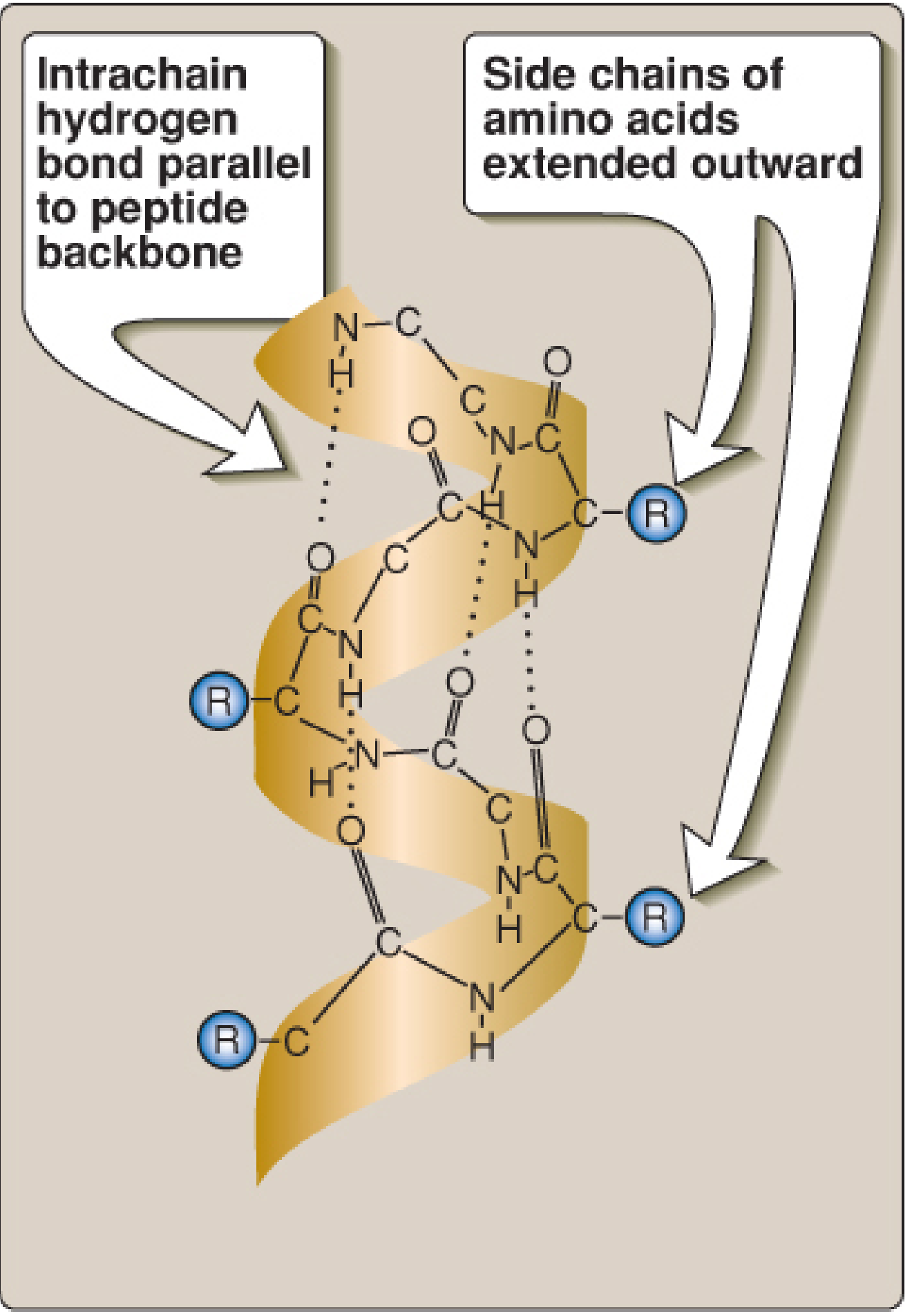
Right-handed spiral composed entirely of L-amino acids
φ ≈ -57°, ψ ≈ -47° (Ramachandran plot, lower left quadrant)
3.6 amino acid residues per turn; pitch (rise per turn) = 0.54 nm
Side chains (R groups) point outward from the central axis to avoid steric interference
Stabilized by hydrogen bonds between the carbonyl oxygen (C=O) of one residue and the amide hydrogen (N-H) of the residue four positions ahead in the chain - these H-bonds run parallel to the helix axis
All peptide bond components participate in H-bonding except those at the very first and last turns
Found abundantly in keratins (hair, skin) and myoglobin

Residues that disrupt α-helices:

Proline - its rigid cyclic secondary amino group cannot adopt the required φ angle; introduces a "kink"
Glycine - too flexible; too many conformations available; destabilizes the helix
Amino acids with bulky or charged R groups (e.g., Trp, Glu) or β-branched residues (Val, Ile) are less compatible

B. The β-Sheet (β-Pleated Sheet)

Key features:

Formed by two or more β-strands aligned laterally; the backbone is nearly fully extended
Stabilized by hydrogen bonds perpendicular to the polypeptide backbone, between the C=O of one strand and the N-H of an adjacent strand (contrast with α-helix where H-bonds are parallel)
Antiparallel β-sheet: adjacent strands run in opposite directions (N→C alternating); H-bonds are more linear and stronger
Parallel β-sheet: adjacent strands run in the same direction (N-termini together); H-bonds are slightly bent; requires chain to loop back via a connecting segment
The surface is pleated ("β-pleated") because successive α-carbons lie slightly above and below the plane
R groups on each β-strand extend alternately above and below the plane of the sheet
β-sheets have a right-handed curl (twist) when viewed along the backbone
R groups can create amphipathic β-sheets (polar and nonpolar faces)

C. β-Turns (β-Bends)

Short loops of 4 amino acids that reverse the direction of the chain, enabling compact globular shape
Usually found on the surface of proteins, often containing charged residues
Frequently connect successive antiparallel β-strands
Often contain proline (causes kink) and glycine (small R group, flexible)
Stabilized by a hydrogen bond between the first and fourth residue in the turn

D. Nonrepetitive Secondary Structure

Loops and coils are regions without a regular repeating pattern. They are not "random" - they have defined conformations but are not periodic. Loops on the protein surface often mediate binding interactions.

E. Supersecondary Structures (Motifs)

Combinations of secondary structure elements form motifs (e.g., β-α-β unit, β-meander, Greek key, helix-loop-helix). Motifs are conserved across proteins with related functions (e.g., helix-loop-helix in DNA-binding transcription factors).

IV. Tertiary Structure

Tertiary structure refers to the complete three-dimensional arrangement of all atoms in a single polypeptide chain - the overall fold. It is determined by the primary structure.

"The primary structure of a polypeptide chain determines its tertiary structure... The tertiary structure of globular proteins in aqueous solution is compact, with a high density (close packing) of the atoms in the core of the molecule. Hydrophobic side chains are buried in the interior, whereas hydrophilic groups are generally found on the surface." - Lippincott, p. 69

Domains

Proteins >200 amino acids usually fold into two or more domains - compact, semi-independent structural and functional units. Each domain folds largely independently and has the properties of a small globular protein.

V. Bonds Stabilizing Tertiary Structure

Four types of interaction cooperate to stabilize the tertiary structure of globular proteins:

Interaction	Nature	Description
Disulfide bonds	Covalent	Formed by oxidation of the -SH (sulfhydryl) groups of two cysteine residues → cystine residue (-S-S-). The strongest stabilizing interaction. Two cysteines may be far apart in primary sequence but brought together by folding. Especially common in secreted/extracellular proteins (e.g., immunoglobulins, insulin).
Hydrophobic interactions	Non-covalent (entropy-driven)	Nonpolar R groups cluster in the interior of the protein, away from aqueous solvent. This is the dominant driving force for protein folding. The aggregation releases ordered water molecules around hydrophobic groups, increasing entropy.
Hydrogen bonds	Non-covalent (electrostatic)	Polar side chains containing O-H or N-H (e.g., Ser, Thr, Asn, Gln) form H-bonds with electron-rich atoms (e.g., carboxylate oxygens, backbone carbonyls). H-bonds on the surface also enhance solubility by interacting with water. Individually weak but collectively strong.
Ionic interactions (salt bridges)	Non-covalent (electrostatic)	Oppositely charged side chains attract each other: e.g., Asp/Glu (-COO⁻) with Lys/Arg (-NH₃⁺). Found on the protein surface and at domain interfaces.

Additional van der Waals forces also contribute to stabilization through transient induced dipole-dipole interactions between tightly packed atoms in the hydrophobic core.

Protein Folding

Folding is a rapid, ordered, non-random process (seconds to minutes). It proceeds through intermediate stages:

Formation of secondary structure driven by the hydrophobic effect - hydrophobic groups aggregate and water is expelled
Combination of secondary elements into larger units
Final native (low-energy) conformation is achieved

Molecular chaperones (e.g., Hsp70, chaperonins) assist folding in vivo by preventing premature aggregation. Protein disulfide isomerase catalyzes the formation and reshuffling of disulfide bonds.

Summary Table: Bonds at Each Level

Structure Level	Stabilizing Bond(s)
Primary	Peptide bonds (covalent)
Secondary (α-helix, β-sheet, β-turn)	Hydrogen bonds (backbone atoms)
Tertiary	Disulfide bonds (covalent), Hydrophobic interactions, Hydrogen bonds (side chains), Ionic interactions, Van der Waals forces

Sources:

Biochemistry, 8th ed., Lippincott Illustrated Reviews, Chapter 2 (pp. 50-75)
Harper's Illustrated Biochemistry, 32nd Ed., Chapters 3 & 5 (pp. 33-34, 46-52)

This is a shared conversation. Sign in to Orris to start your own chat.