
explain the normal curve for a theory mbbs exam, with reference from K Park’s book of preventive and social medicine
Reading File
The normal curve is a bell-shaped frequency distribution fundamental to biostatistics. Let me search K Park's textbook directly.
Searching sources...
Finding Sources
Finding Sources
Found the exact sections in K Park. Now let me read all relevant content in one go.
Reading File
Reading File
Loading Image
I now have all the content directly from K Park. Here is the complete explanation:
The Normal Curve - as per K Park's Textbook of Preventive and Social Medicine
1. Definition
"The normal distribution or 'normal curve' is an important concept in statistical theory."
- Park's Textbook of Preventive and Social Medicine, p. 953
If you collect haemoglobin values from a very large number of people and make a frequency distribution with narrow class intervals, you get a smooth, symmetrical bell-shaped curve - this is the normal distribution or normal curve. The exact shape depends on the mean (x̄) and standard deviation (σ) of the data, so theoretically there is an infinite number of normal curves.
2. The Normal Curve (Fig. 15 - K Park)
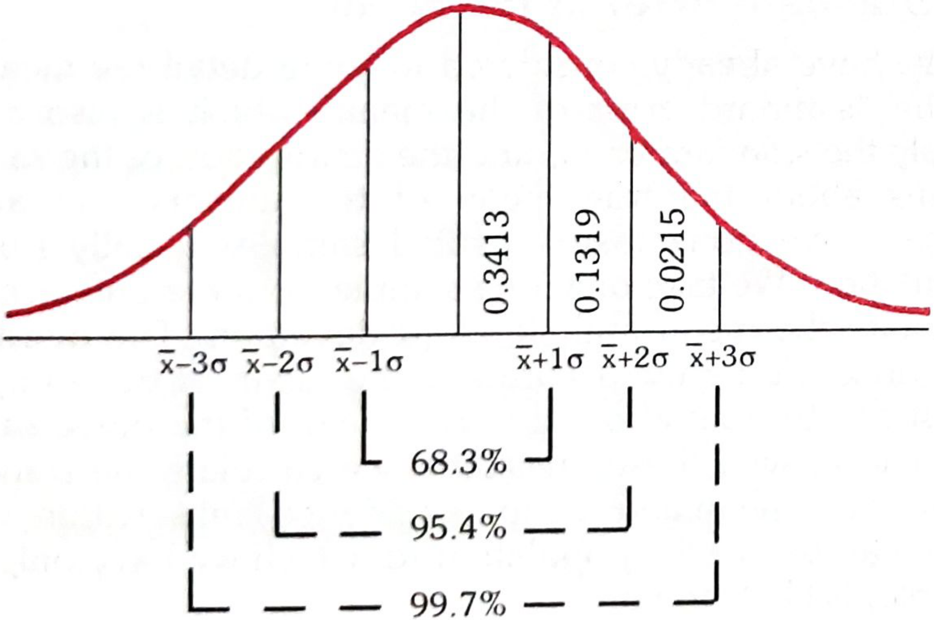
FIG. 15 - Normal Curve (Park's Textbook of Preventive and Social Medicine)
3. Key Properties and the 68-95-99.7 Rule
This is the single most important thing to memorize for your theory exam:
| Range | Area under curve | % Values included | Confidence |
|---|---|---|---|
| x̄ ± 1σ | 0.6827 | 68.3% | - |
| x̄ ± 2σ | 0.9545 | 95.4% (~95%) | 95% confidence limits |
| x̄ ± 3σ | 0.9973 | 99.7% | - |
The areas in each half-segment (right side of mean) as shown in Fig. 15:
- Between x̄ and x̄+1σ: 0.3413 (34.13%)
- Between x̄+1σ and x̄+2σ: 0.1319 (13.19%)
- Between x̄+2σ and x̄+3σ: 0.0215 (2.15%)
(By symmetry, the same proportions apply on the left side.)
4. Confidence Limits
The limits on either side of the mean that include a stated percentage of values are called confidence limits.
"The probability of a reading falling outside the 95% confidence limits is 1 in 20 (P = 0.05)."
- Park's, p. 953
- 95% confidence limits = x̄ ± 2σ → P = 0.05 that a value falls outside
- 99.7% confidence limits = x̄ ± 3σ → P = 0.003 that a value falls outside
5. The Standard Normal Curve
Because there are infinite normal curves, statisticians devised one standardized normal curve to calculate areas under any normal curve.
Properties of the Standard Normal Curve:
- Smooth, bell-shaped, perfectly symmetrical
- Based on an infinitely large number of observations
- Total area = 1
- Mean = 0
- Standard deviation (σ) = 1
- Mean, median, and mode all coincide at the centre
The Z-score (Standard Normal Deviate)
The distance of a value (x) from the mean in units of standard deviation is called the relative deviate or standard normal variate, denoted by Z:
$$Z = \frac{x - \bar{x}}{\sigma}$$
When a variable x is converted to Z, it is said to be standardized - its mean becomes 0 and its standard deviation becomes 1.
6. Areas Under the Standard Normal Curve (Table 4 - K Park)
| Relative deviate (Z) | Proportion of area from middle of curve |
|---|---|
| 0.00 | 0.0000 |
| 0.50 | 0.1915 |
| 1.00 | 0.3413 |
| 1.50 | 0.4332 |
| 2.00 | 0.4772 |
| 3.00 | 0.4987 |
| 4.00 | 0.49997 |
| 5.00 | 0.4999998 |
Table 4, Park's Textbook of Preventive and Social Medicine
7. Worked Example from K Park (Estimation of Probability)
"Let us suppose, the pulse of a group of normal healthy males was 72, with a standard deviation of 2. What is the probability that a male chosen at random would be found to have a pulse of 80 or more?"
Step 1: Calculate Z:
$$Z = \frac{x - \bar{x}}{\sigma} = \frac{80 - 72}{2} = 4$$
Step 2: From Table 4, area corresponding to Z = 4 is 0.49997
Step 3: Since we want the area beyond Z = 4 (the tail), we subtract from 0.5 (half the total area):
$$0.5 - 0.49997 = 0.00003$$
Conclusion: The probability is that only 3 out of 100,000 individuals would have a pulse rate of 80 or higher.
Quick Exam Summary
| Point | Value |
|---|---|
| Shape | Bell-shaped, symmetrical |
| Mean = Median = Mode | Yes (all coincide) |
| x̄ ± 1σ | 68.3% of values |
| x̄ ± 2σ | 95.4% of values (P = 0.05 outside) |
| x̄ ± 3σ | 99.7% of values |
| Standard normal curve: Mean | 0 |
| Standard normal curve: SD | 1 |
| Standard normal curve: Total area | 1 |
| Z formula | (x - x̄) / σ |
Reference: Park K. Park's Textbook of Preventive and Social Medicine, Chapter on Biostatistics, pp. 953-954 (Standard Normal Curve and Normal Distribution).
This is a shared conversation. Sign in to Orris to start your own chat.