
Detailed 20 marks answer for University biostatistics exams Biostatistics and branches of biostatistics
Reading File
Finding Sources
Finding Sources
Finding Sources
Finding Sources
Finding Sources
Finding Sources
Reading File
Finding Sources
Reading File
Finding Sources
I have enough material from the textbooks. Now I'll compose the full 20-mark university exam answer.
Biostatistics and Branches of Biostatistics
1. Introduction
The word "biostatistics" is a combination of two Greek words - bios (life) and statistikos (pertaining to the state). Biostatistics is the science of applying statistical reasoning and methods to biological, medical, and public health data. It serves as the backbone of evidence-based medicine, allowing researchers, clinicians, and public health workers to collect, organize, analyze, interpret, and present health-related data in a meaningful way.
Without biostatistics, no clinical trial could determine whether a new drug works, no epidemiologist could track disease spread, and no public health policy could be grounded in evidence. As stated in Barash, Cullen, and Stoelting's Clinical Anesthesia (9th ed.): "The language of medicine is increasingly statistical. Without exception, physicians must read the language of science to independently assess and interpret the scientific report."
2. Definitions
Narrow Definition
Biostatistics is the application of statistical methods to data arising from biological experiments and medical/health investigations.
Broad Definition (Park's Textbook of Preventive and Social Medicine)
Biostatistics is the science that deals with the collection, compilation, tabulation, analysis, and interpretation of numerical (quantitative) data relating to biological phenomena - especially in the fields of medicine, public health, and life sciences.
Statistics vs. Biostatistics
| Feature | Statistics | Biostatistics |
|---|---|---|
| Scope | General (economics, engineering, etc.) | Biological and health sciences |
| Data type | Any quantitative data | Biological, clinical, epidemiological data |
| Purpose | General inference | Health policy, clinical decisions, disease control |
3. Importance of Biostatistics
Biostatistics is important because:
- Planning research - helps define the hypothesis, select study design, and calculate sample size
- Analyzing clinical trials - determines whether an intervention is effective
- Epidemiology - measures disease frequency, risk factors, and associations
- Health policy - mortality rates, birth rates, and disease burden inform resource allocation
- Evidence-based medicine - systematic reviews and meta-analyses depend entirely on statistical synthesis
- Quality control - monitoring hospital infection rates, surgical outcomes
- Demography and vital statistics - tracking population changes, births, deaths, migration
4. Basic Terminology
- Population: The entire group of individuals about which information is desired
- Sample: A subset of the population selected for study
- Variable: Any characteristic that can take different values (e.g., blood pressure, age)
- Data: Observed values of a variable
- Parameter: A numerical summary of the population
- Statistic: A numerical summary of the sample
Types of Variables
| Type | Subtype | Examples |
|---|---|---|
| Qualitative (Categorical) | Nominal | Blood group, gender, religion |
| Qualitative (Categorical) | Ordinal | Pain scale (mild, moderate, severe) |
| Quantitative (Numerical) | Discrete | Number of pregnancies, parity |
| Quantitative (Numerical) | Continuous | Blood pressure, height, temperature |
5. Branches of Biostatistics
Biostatistics is a broad discipline with several specialized branches, each serving distinct functions in health and biological sciences.
Branch 1: Descriptive Statistics
Definition: The branch that summarizes and describes the features of a dataset without drawing conclusions beyond the data itself.
Key tools:
- Measures of Central Tendency: Mean (arithmetic average), Median (middle value), Mode (most frequent value)
- Measures of Dispersion: Range, Standard Deviation (SD), Variance, Coefficient of Variation (CV)
- Graphical methods: Bar charts, pie charts, histograms, frequency polygons, box-and-whisker plots
- Tabulation: Frequency tables, relative frequency
Example in medicine: Reporting that the mean systolic blood pressure in a study group was 128 mmHg ± 10 mmHg (SD) is a descriptive statistic.
Clinical Anesthesia states: "The use of graphs, descriptive statistics (e.g., mean, standard deviation), and inferential statistics (e.g., t-test, confidence interval) are important methods for the presentation of research results."
Branch 2: Inferential Statistics
Definition: The branch that uses sample data to draw conclusions (inferences) about a larger population, with a quantified degree of uncertainty.
Key tools:
- Hypothesis testing: Null hypothesis (H₀) vs. Alternative hypothesis (H₁)
- Parametric tests: Student's t-test, ANOVA (Analysis of Variance), Pearson correlation, linear regression
- Non-parametric tests: Mann-Whitney U test, Kruskal-Wallis test, Chi-square test
- Confidence intervals: A range of values within which the true population parameter likely falls
- p-value: Probability of obtaining results as extreme as observed, assuming H₀ is true (significance threshold usually p < 0.05)
Two main schools:
- Frequentist statistics: Conclusions based only on observed data
- Bayesian statistics: Incorporates prior knowledge along with observed data
Example in medicine: A t-test used to compare mean cholesterol levels between a treated group and a control group in a drug trial is inferential statistics.
Branch 3: Vital Statistics
Definition: The systematic collection, analysis, and interpretation of data on vital events - births, deaths, marriages, divorces, and disease notifications.
Sources of vital statistics:
- Civil registration systems (birth and death registration)
- Census data
- Hospital records
- Notifiable disease reports
- Sample Registration System (SRS)
Key vital statistics indicators:
- Crude Birth Rate (CBR): Number of live births per 1,000 population per year
- Crude Death Rate (CDR): Number of deaths per 1,000 population per year
- Infant Mortality Rate (IMR): Deaths under 1 year per 1,000 live births
- Maternal Mortality Ratio (MMR): Maternal deaths per 100,000 live births
- Life Expectancy at Birth: Average number of years a newborn is expected to live
Importance: Vital statistics form the backbone of health planning and resource allocation by governments and international bodies (WHO, UNICEF).
As noted in Park's Textbook of Preventive and Social Medicine, the components of a health information system must include "demography and vital events; environmental health statistics; health status (mortality, morbidity, disability, quality of life); health resources (facilities, beds, manpower)."
Branch 4: Epidemiological Statistics (Epidemiostatistics)
Definition: The application of statistical methods to epidemiological studies to measure disease frequency, study risk factors, and evaluate the association between exposures and outcomes.
Key measures:
- Prevalence: Proportion of a population with a disease at a given time
- Incidence rate: Number of new cases per unit population per unit time
- Relative Risk (RR): Risk in exposed group / Risk in unexposed group (used in cohort studies)
- Odds Ratio (OR): Odds of exposure in cases / Odds of exposure in controls (used in case-control studies)
- Attributable Risk (AR): Excess risk due to a specific exposure
- Number Needed to Treat (NNT): Number of patients treated to prevent one outcome
Study designs using epidemiological statistics:
- Cross-sectional studies
- Case-control (retrospective) studies
- Cohort (prospective) studies
- Ecological studies
- Randomized Controlled Trials (RCTs)
Branch 5: Demography
Definition: The statistical study of human populations, including their size, structure, distribution, and dynamics (births, deaths, migration).
Key demographic measures:
- Age-sex pyramid (population pyramid)
- Dependency ratio
- Fertility rate (Total Fertility Rate - TFR)
- Net Reproduction Rate (NRR)
- Population growth rate
- Standardized mortality/morbidity ratios
Types of demographic studies:
- Formal demography: Mathematical and statistical analysis of population data
- Social demography: Interaction between demographic variables and social factors (income, education, religion)
Application: Demographic data guides health workforce planning, vaccine procurement, and hospital bed allocation.
Branch 6: Clinical Biostatistics (Clinical Trial Statistics)
Definition: The application of statistical principles specifically to the design, conduct, analysis, and interpretation of clinical trials and medical research.
Key concepts:
- Sample size calculation: Power of a study (usually 80-90%), Type I error (α = 0.05), Type II error (β = 0.20)
- Randomization: Ensures equal distribution of confounding variables between groups
- Blinding: Single-blind (patient unaware), Double-blind (patient + investigator unaware), Triple-blind (including data analyst)
- Intention-to-treat (ITT) analysis: Analyzes patients in the group they were randomized to, regardless of protocol deviation
- Per-protocol analysis: Analyzes only patients who completed the trial as planned
Trial phases:
- Phase I: Safety and dosing (small healthy volunteers)
- Phase II: Efficacy and side effects (small patient groups)
- Phase III: Large-scale efficacy comparison with standard treatment
- Phase IV: Post-marketing surveillance
Clinical Anesthesia notes: "Good research planning includes a clear biologic hypothesis, the specification of outcome variables, the choice of anticipated statistical methods, and sample size planning."
Branch 7: Survival Analysis
Definition: A branch dealing with time-to-event data, particularly the time from start of follow-up until a defined event (death, disease recurrence, recovery) occurs.
Key tools:
- Kaplan-Meier curves: Graphical display of survival probability over time
- Log-rank test: Compares survival between two or more groups
- Cox proportional hazards regression: Identifies risk factors affecting time-to-event
- Hazard ratio (HR): The relative risk of the event at any point in time
Application: Used extensively in cancer research (5-year survival rates), HIV/AIDS research, and cardiovascular outcome trials.
Branch 8: Systematic Reviews and Meta-analysis
Definition: Statistical methods for combining results from multiple independent studies to reach more powerful and reliable conclusions.
Process:
- Systematic literature search (PubMed, Cochrane, EMBASE)
- Quality assessment of included studies (GRADE criteria, Cochrane risk-of-bias tool)
- Data extraction and pooling using weighted average
- Forest plot: Graphical display of individual and pooled effect sizes
- Funnel plot: Assessment of publication bias
Key statistics:
- Pooled Risk Ratio / Odds Ratio / Mean Difference
- Heterogeneity (I² statistic): I² > 50% indicates substantial heterogeneity
- Random effects model vs. Fixed effects model
Clinical Anesthesia states: "Systematic review and meta-analysis summarize the results of individual studies and permit more powerful inferences for the comparison of interventions."
Branch 9: Health Statistics (Medical Statistics)
Definition: Collection and analysis of statistics specifically pertaining to health services - hospital utilization, disease burden, healthcare quality, and health system performance.
Examples:
- Bed occupancy rate
- Average length of hospital stay
- Surgical site infection rates
- Readmission rates
- Disease-specific mortality rates
Organizations maintaining health statistics:
- World Health Organization (WHO) - Global Health Observatory
- National Health Profile (India)
- Centers for Disease Control and Prevention (CDC) - USA
- Office of National Statistics (ONS) - UK
6. Relationship Between the Branches
             BIOSTATISTICS
                  |
    ┌─────────────┼─────────────┐
    |             |             |
Descriptive   Inferential   Vital Statistics
Statistics    Statistics         |
    |             |         Demography
  Graphs     Hypothesis         |
  Tables      Testing       Health Planning
    |             |
Epidemio-    Clinical
statistics   Biostatistics
    |             |
  Risk       Clinical Trials
Measures    Meta-analysis
                  |
           Survival Analysis
7. Applications of Biostatistics
| Field | Application |
|---|---|
| Clinical Medicine | Drug efficacy trials, diagnostic test evaluation |
| Public Health | Disease surveillance, vaccination program evaluation |
| Epidemiology | Disease outbreaks, risk factor identification |
| Genetics | Gene frequency, Hardy-Weinberg equilibrium |
| Nursing | Patient outcomes research, care quality metrics |
| Pharmacology | Dose-response relationships, adverse drug reactions |
| Dentistry | Caries prevalence, treatment outcome studies |
| Nutrition | Dietary assessment, micronutrient deficiency surveys |
8. Limitations of Biostatistics
- A statistical association does not prove causation (e.g., correlation does not equal causation)
- Results depend entirely on the quality and representativeness of the sample - garbage in, garbage out
- p-values can be misleading; clinical significance and statistical significance can differ
- Biological variation is high, making precise predictions difficult
- Requires expertise - misuse of statistical tests leads to erroneous conclusions
- Cannot account for all confounding variables in observational studies
9. Summary Table: Branches of Biostatistics
| Branch | Focus | Key Tools |
|---|---|---|
| Descriptive Statistics | Summarizing data | Mean, SD, tables, graphs |
| Inferential Statistics | Population conclusions from samples | t-test, ANOVA, chi-square, p-value |
| Vital Statistics | Birth, death, disease events | CBR, CDR, IMR, MMR |
| Demography | Population structure and dynamics | TFR, population pyramid |
| Epidemiological Statistics | Disease frequency and risk | RR, OR, incidence, prevalence |
| Clinical Biostatistics | Clinical trial design and analysis | Sample size, randomization, blinding |
| Survival Analysis | Time-to-event data | Kaplan-Meier, Cox regression |
| Meta-analysis | Pooling multiple studies | Forest plot, I², pooled OR |
| Health Statistics | Health service performance | Bed occupancy, length of stay |
10. Conclusion
Biostatistics is not merely a mathematical tool - it is the scientific foundation of modern medicine, public health, and biological research. Its branches collectively enable clinicians to design sound experiments, epidemiologists to quantify disease burden, public health professionals to evaluate interventions, and policymakers to allocate resources rationally. A thorough understanding of biostatistics is therefore indispensable for any healthcare professional or researcher aiming to practice and advance evidence-based medicine.
References used:
- Barash, Cullen, and Stoelting's Clinical Anesthesia, 9th Edition - Chapter on Experimental Medicine & Data Analysis
- Park's Textbook of Preventive and Social Medicine - Chapter on Health Information Systems
- The Harriet Lane Handbook (Johns Hopkins), 23rd Ed. - Section on Biostatistics and Evidence-Based Medicine
Explain descriptive and inferential with detailed example
Finding Sources
Finding Sources
Reading File
Reading File
Reading File
Reading File
Excellent - I have rich textbook content. Now I'll compose the full detailed answer.
Descriptive and Inferential Statistics - Detailed Explanation with Examples
PART A: DESCRIPTIVE STATISTICS
1. Definition
Descriptive statistics is the branch of statistics that organizes, summarizes, and presents data in a meaningful and informative way - without drawing conclusions beyond the data at hand. The goal is purely to describe what is in the sample.
As stated in Henry's Clinical Diagnosis and Management by Laboratory Methods:
"The quantification of information in meaningful summaries and comparisons is the domain of statistical analysis. Descriptive statistics provide a consistent framework for calculating or estimating the central tendency of continuous data in the familiar forms of mean, median, and mode. The variation in data is generally described by the mathematical calculations of variances and standard deviations."
2. Components of Descriptive Statistics
Descriptive statistics has two main components: Measures of Central Tendency and Measures of Dispersion.
A. Measures of Central Tendency
These describe the "center" or "typical value" of a dataset.
| Measure | Definition | When to Use |
|---|---|---|
| Mean | Sum of all values / Number of observations | Normally distributed, continuous data |
| Median | The middle value when data is arranged in order | Skewed data, ordinal data |
| Mode | The most frequently occurring value | Nominal (categorical) data, bimodal distributions |
From Rockwood and Green's Fractures in Adults (10th ed., 2025):
"The sample mean is equal to the sum of the measurements divided by the number of observations. The median of a set of measurements is the number that falls in the middle. The mode is the most frequently occurring number in a set of measurements."
Choosing the right measure:
- If data is normally distributed (bell-shaped) → use Mean
- If data is skewed or has outliers → use Median
- If data is categorical → use Mode
From Cummings Otolaryngology:
"Another way is to examine the SD; when it is very large (e.g., larger than the mean value with which it is associated), the data often have an asymmetric distribution and should be described by the median and interquartile range. When in doubt, the median should always be used over the mean."
B. Measures of Dispersion (Spread)
These describe how spread out the data values are around the center.
| Measure | Definition | Use |
|---|---|---|
| Range | Largest value - Smallest value | Simple, but sensitive to outliers |
| Standard Deviation (SD) | Average distance of each value from the mean | Symmetric/normal data |
| Variance | SD squared | Used in statistical calculations |
| Interquartile Range (IQR) | 75th percentile - 25th percentile | Skewed data; resistant to outliers |
| Coefficient of Variation (CV) | (SD / Mean) × 100% | Comparing variability across different units |
| Percentile | % of values equal to or below a number | Growth charts, lab reference ranges |
From Henry's Clinical Diagnosis:
"Coefficient of variation (CV) is the standard deviation of a set of data points divided by the mean result expressed as a percentage or as a decimal fraction."
C. Graphical / Visual Descriptive Tools
- Bar chart - for categorical data (e.g., blood groups in a ward)
- Histogram - for continuous data (e.g., distribution of ages)
- Pie chart - proportions of a whole
- Box-and-whisker plot - shows median, IQR, and outliers
- Frequency polygon - shape of distribution
- Scatter plot - relationship between two continuous variables
3. Normal Distribution and the 68-95-99.7 Rule
When data follows a normal (bell-shaped) distribution:
- 68% of values fall within 1 SD of the mean
- 95% fall within 2 SD
- 99.7% fall within 3 SD
This is the basis of setting reference ranges in clinical laboratories (mean ± 2 SD covers 95% of healthy individuals).
4. Detailed Worked Example - Descriptive Statistics
Scenario: A medical student collects fasting blood glucose values (mg/dL) from 10 patients in a diabetic clinic:
| Patient | Glucose (mg/dL) |
|---|---|
| 1 | 95 |
| 2 | 110 |
| 3 | 126 |
| 4 | 98 |
| 5 | 140 |
| 6 | 105 |
| 7 | 126 |
| 8 | 112 |
| 9 | 88 |
| 10 | 100 |
Step 1 - Sort the data (ascending order):
88, 95, 98, 100, 105, 110, 112, 126, 126, 140
Step 2 - Calculate the Mean:
Mean = (88 + 95 + 98 + 100 + 105 + 110 + 112 + 126 + 126 + 140) / 10
= 1100 / 10 = 110 mg/dL
Step 3 - Calculate the Median:
n = 10 (even), so median = average of 5th and 6th values
= (105 + 110) / 2 = 107.5 mg/dL
Step 4 - Find the Mode:
126 appears twice → Mode = 126 mg/dL
Step 5 - Range:
= 140 - 88 = 52 mg/dL
Step 6 - Standard Deviation:
Deviations from mean (110): -22, -15, -12, -10, -5, 0, +2, +16, +16, +30
Squared deviations: 484, 225, 144, 100, 25, 0, 4, 256, 256, 900
Sum = 2394
Variance = 2394 / (10 - 1) = 266.0
SD = √266.0 ≈ 16.3 mg/dL
Step 7 - Interpretation:
The 10 patients had a mean fasting glucose of 110 ± 16.3 mg/dL (Mean ± SD), a median of 107.5 mg/dL, and a range of 88-140 mg/dL. The mean is close to the median, suggesting the data is approximately normally distributed. No outlier significantly distorts the mean. This is purely a description of the sample - no inference about any larger population is made yet.
PART B: INFERENTIAL STATISTICS
1. Definition
Inferential statistics uses data from a sample to draw conclusions (inferences) about the larger population from which the sample was drawn. Because we rarely have access to entire populations, we estimate population parameters from sample statistics, always acknowledging a degree of uncertainty.
From Rockwood and Green's Fractures in Adults (2025):
"In comparative research designs, the primary question is typically 'which treatment is superior?' Answering this question in an objective and quantitative manner requires statistical inference. Much like a criminal trial, which commences with a fundamental presumption of innocence - a comparative study commences with a fundamental presumption of 'no difference,' known as the null hypothesis."
2. Core Concepts in Inferential Statistics
A. Hypothesis Testing - Step by Step
| Step | Action |
|---|---|
| 1 | State the Null Hypothesis (H₀): No difference / no effect |
| 2 | State the Alternative Hypothesis (H₁): There is a difference / effect |
| 3 | Choose a significance level (α) - usually 0.05 (5%) |
| 4 | Select the appropriate statistical test |
| 5 | Calculate the test statistic and p-value |
| 6 | Decision: If p < α → Reject H₀ (result is statistically significant) |
B. The p-value
The p-value is the probability of obtaining results at least as extreme as observed, assuming the null hypothesis is true.
- p < 0.05: Statistically significant - reject H₀
- p ≥ 0.05: Not statistically significant - fail to reject H₀
- p < 0.01: Highly significant
- p < 0.001: Very highly significant
From Rockwood and Green's:
"If the probability of the null hypothesis being true falls below a certain reasonable (albeit arbitrary) threshold, we can conclude that the two treatments likely differ. In the medical literature, this threshold is typically set at a value of less than 5% (i.e., p < .05)."
Coin toss analogy (from the same textbook):
"A coin tossed 10 times, landing heads all 10 times has a probability of 0.5¹⁰ ≈ p < 0.001. Therefore the null hypothesis (fair coin) is rejected - the result is 'statistically significant.'"
C. Type I and Type II Errors
| Error | Definition | Symbol | Consequence |
|---|---|---|---|
| Type I (α) | Rejecting H₀ when it is actually true | α = 0.05 | False positive - claim a treatment works when it doesn't |
| Type II (β) | Failing to reject H₀ when it is actually false | β = 0.20 | False negative - miss a real treatment effect |
| Power (1-β) | Probability of correctly detecting a true effect | Usually 0.80 | Adequate power avoids missing real effects |
D. Confidence Interval (CI)
A confidence interval gives a range of plausible values for the true population parameter.
From Henry's Clinical Diagnosis:
"Confidence interval (CI) is the interval that is computed to include a parameter such as the mean with a stated probability (e.g., commonly 90%, 95%, 99%) that the true value falls into that interval."
- A 95% CI means: if we repeated the study 100 times, 95 of those intervals would contain the true population mean.
- Narrow CI = more precise estimate (larger sample)
- Wide CI = less precise (smaller sample)
Practical rule: If a 95% CI for a difference between two groups does not cross zero (or 1.0 for ratio measures), the result is statistically significant at p < 0.05.
3. Choosing the Right Statistical Test
For Comparing Groups (Parametric - assumes normal distribution):
| Situation | Test |
|---|---|
| Compare 2 independent group means | Independent samples t-test |
| Compare same group before and after | Paired t-test |
| Compare 3 or more group means | One-way ANOVA |
| Association between 2 continuous variables | Pearson's correlation / Linear regression |
For Non-parametric Data (skewed, ordinal, or small samples):
| Situation | Test |
|---|---|
| Compare 2 independent groups | Mann-Whitney U test |
| Compare same group before and after | Wilcoxon signed-rank test |
| Compare 3+ groups | Kruskal-Wallis test |
| Association between ordinal variables | Spearman's rank correlation |
For Categorical Data:
| Situation | Test |
|---|---|
| Compare proportions between 2+ groups | Chi-square (χ²) test |
| Small expected cell frequencies (< 5) | Fisher's exact test |
| Paired categorical data | McNemar's test |
From Henry's Clinical Diagnosis:
"Comparison of data typically asks the question whether one group is different from another group. These comparisons are usually done by t-test or by analysis of variance depending on whether two or more groups of continuous data are compared. If the data are discrete, comparison is done by chi-square analysis."
4. Detailed Worked Example - Inferential Statistics
Scenario: A researcher wants to test whether a new antihypertensive drug (Drug A) lowers systolic blood pressure (SBP) significantly more than a placebo.
- Group 1 (Drug A): 30 hypertensive patients → Mean SBP after treatment = 128 mmHg, SD = 10 mmHg
- Group 2 (Placebo): 30 hypertensive patients → Mean SBP after treatment = 140 mmHg, SD = 12 mmHg
Step 1 - State the Hypotheses:
- H₀: There is no difference in mean SBP between Drug A and placebo (μ₁ = μ₂)
- H₁: Drug A significantly lowers mean SBP compared to placebo (μ₁ ≠ μ₂)
Step 2 - Choose significance level:
- α = 0.05 (5%)
Step 3 - Select the test:
- Two independent groups, continuous data, approximately normal → Independent samples t-test
Step 4 - Calculate the test statistic (t):
Difference in means = 140 - 128 = 12 mmHg

Standard Error (SE) = √[(SD₁²/n₁) + (SD₂²/n₂)]
                    = √[(100/30) + (144/30)]
                    = √[3.33 + 4.80]
                    = √8.13 ≈ 2.85

t = Difference / SE = 12 / 2.85 ≈ 4.21
Step 5 - Find the p-value:
With degrees of freedom (df) ≈ 58, a t-value of 4.21 gives p < 0.001
Step 6 - Calculate 95% Confidence Interval:
95% CI = Difference ± (1.96 × SE)
       = 12 ± (1.96 × 2.85)
       = 12 ± 5.59
       = (6.41 to 17.59 mmHg)
Step 7 - Interpret the results:
"The mean SBP was significantly lower in the Drug A group (128 ± 10 mmHg) compared to the placebo group (140 ± 12 mmHg). The mean difference was 12 mmHg (95% CI: 6.4 to 17.6 mmHg; p < 0.001). The null hypothesis is rejected. Drug A produces a statistically significant reduction in systolic blood pressure."
Statistical significance vs. Clinical significance:
The 95% CI (6.4 to 17.6 mmHg) does not cross zero, confirming statistical significance. A reduction of 12 mmHg in SBP is also clinically meaningful - every 10 mmHg reduction in SBP reduces cardiovascular risk by approximately 20-25%. In this case, statistical significance and clinical significance align.
This concept is highlighted in Rockwood and Green's:
"Two competing treatments may produce statistically different outcomes, but the calculated difference may still fail to reach the threshold for clinical importance (i.e., the MCID)... Despite the statistically significant difference, the conclusion must be that there is no clinical advantage."
PART C: COMPARISON - Descriptive vs. Inferential Statistics
| Feature | Descriptive Statistics | Inferential Statistics |
|---|---|---|
| Purpose | Summarize and describe the data | Draw conclusions about a population from a sample |
| Scope | Applies only to the data collected | Extends beyond the sample to the population |
| Output | Mean, SD, median, graphs, tables | p-value, t-statistic, CI, OR, RR |
| Conclusion | "What does this data look like?" | "Is there a real effect in the population?" |
| Uncertainty | No uncertainty quantified | Uncertainty explicitly quantified (CI, p-value) |
| Examples | Mean BP = 128 mmHg, SD = 10 | p < 0.001; 95% CI: 6.4 - 17.6 mmHg |
| Tests used | None (summary measures only) | t-test, ANOVA, chi-square, regression |
| Use in research | Table 1 (baseline characteristics) | Results section (treatment comparisons) |
PART D: How They Work Together in Practice
In any well-designed clinical study, both types of statistics are used sequentially:
-
Descriptive statistics first - characterize the study population (Table 1: age, gender, baseline BP, comorbidities). This helps assess whether the groups are comparable before treatment.
-
Inferential statistics second - test the primary and secondary hypotheses and quantify uncertainty (Tables 2-3: treatment outcomes, p-values, CIs).
From Rockwood and Green's Fractures in Adults:
"While descriptive studies may report descriptive statistics as an end per se, analytic studies generally use descriptive statistics to outline the baseline characteristics of participants. This summary of baseline characteristics is critical to readers' assessment of prognostic balance between groups."
Summary
- Descriptive statistics = a photograph of your data (what is)
- Inferential statistics = a telescope aimed at the population (what likely is, with measured uncertainty)
- Both are essential: you cannot make valid inferences without first accurately describing your data
- In medicine, the goal is not just statistical significance (p-value) but clinical significance (does the difference matter to the patient?)
References:
- Rockwood and Green's Fractures in Adults, 10th ed., 2025 - Statistical Inference chapter
- Henry's Clinical Diagnosis and Management by Laboratory Methods - Statistics in Laboratory Medicine
- Cummings Otolaryngology Head and Neck Surgery - Habit 2: Describe Before You Analyze
Just normal example is enough
Got it! Here's a simple, clean explanation with everyday examples.
Descriptive Statistics
Definition: Summarizes and describes the data you have collected. Nothing more, nothing less.
Simple Example:
A nurse measures the weight (kg) of 5 patients:
50, 60, 70, 80, 90
| Measure | Calculation | Result |
|---|---|---|
| Mean | (50+60+70+80+90) / 5 | 70 kg |
| Median | Middle value | 70 kg |
| Mode | No repeat values | None |
| Range | 90 - 50 | 40 kg |
| SD | Spread around mean | ≈ 15.8 kg |
Conclusion (Descriptive):
"The average weight of these 5 patients is 70 kg with a standard deviation of 15.8 kg."
You are only describing what you see. No predictions. No comparisons. No conclusions beyond these 5 patients.
Inferential Statistics
Definition: Uses the sample data to make conclusions about a larger population, with a measured degree of uncertainty (p-value, confidence interval).
Same Example Extended:
Now the researcher asks: "Is the average weight of ALL patients in this hospital different from the national average of 65 kg?"
- Sample mean = 70 kg
- National average (H₀) = 65 kg
- Run a one-sample t-test
- Result: p = 0.03 (less than 0.05)
- 95% CI: (66 to 74 kg)
Conclusion (Inferential):
"The mean weight of patients in this hospital (70 kg) is significantly higher than the national average of 65 kg (p = 0.03). The 95% CI of 66-74 kg does not include 65 kg, confirming the finding."
You are now drawing a conclusion about the whole hospital population based on just 5 patients.
Key Difference in One Line
| Descriptive | Inferential | |
|---|---|---|
| Question | "What does my data show?" | "What does my data tell me about the population?" |
| Output | Mean, SD, tables, graphs | p-value, CI, t-test result |
| Goes beyond sample? | ❌ No | ✅ Yes |
Simple memory trick:
- Descriptive = Describe what's in front of you (like describing a photo)
- Inferential = Infer what's true for everyone (like predicting the weather from a sample reading)
Medical examples
Here you go — clean medical examples for both.
Descriptive Statistics — Medical Example
Scenario: A doctor records the fasting blood sugar (FBS) of 8 diabetic patients in a clinic:
Values (mg/dL): 110, 126, 140, 98, 160, 126, 115, 125
| Measure | Calculation | Result |
|---|---|---|
| Mean | Sum / 8 | 125 mg/dL |
| Median | Average of 4th & 5th values (sorted) | 125.5 mg/dL |
| Mode | 126 appears twice | 126 mg/dL |
| Range | 160 - 98 | 62 mg/dL |
| SD | Spread around mean | ≈ 18.6 mg/dL |
Descriptive Conclusion:
"The 8 diabetic patients had a mean fasting blood sugar of 125 ± 18.6 mg/dL, with values ranging from 98 to 160 mg/dL."
That's it. You are only describing those 8 patients. No further conclusion.
Inferential Statistics — Medical Example
Scenario: A doctor wants to know: "Does Drug A lower blood pressure more than Drug B?"
- Group 1 (Drug A) — 30 patients → Mean SBP = 128 mmHg
- Group 2 (Drug B) — 30 patients → Mean SBP = 140 mmHg
Step 1 — Hypotheses:
- H₀: No difference between Drug A and Drug B
- H₁: Drug A lowers BP more than Drug B
Step 2 — Test used: Independent samples t-test (two groups, continuous data)
Step 3 — Result:
- Difference = 12 mmHg
- p = 0.001 (less than 0.05 → statistically significant)
- 95% CI: 6 to 18 mmHg (does not cross zero → confirms significance)
Inferential Conclusion:
"Drug A significantly reduced systolic blood pressure compared to Drug B by 12 mmHg (p = 0.001, 95% CI: 6–18 mmHg). H₀ is rejected. This result applies to the broader hypertensive population, not just these 60 patients."
Another Quick Medical Example — Chi-square (Inferential)
Scenario: Is smoking associated with lung cancer?
| Lung Cancer | No Lung Cancer | |
|---|---|---|
| Smokers | 70 | 30 |
| Non-smokers | 20 | 80 |
- Test used: Chi-square test (categorical data)
- Result: p < 0.001
Conclusion:
"There is a statistically significant association between smoking and lung cancer (p < 0.001). Smokers are significantly more likely to develop lung cancer."
Side-by-Side Comparison
| Descriptive | Inferential | |
|---|---|---|
| Example | Mean FBS = 125 mg/dL in 8 patients | Drug A lowers BP more than Drug B (p = 0.001) |
| What it does | Describes the sample | Concludes about the population |
| Tools used | Mean, SD, range, median | t-test, chi-square, p-value, 95% CI |
| Goes beyond sample? | ❌ No | ✅ Yes |
One-line memory aid:
- Descriptive → "Here is what I found in MY patients."
- Inferential → "Here is what this means for ALL patients like them."
Next question for 20 marks measures of central tendency
Finding Sources
Finding Sources
Reading File
Reading File
Reading File
Reading File
Loading Image
Loading Image
Now I have everything needed. Here is the complete 20-mark answer.
Measures of Central Tendency
1. Introduction
In any statistical investigation, a researcher collects a large number of observations. To make sense of this data, it is necessary to find a single representative value that best describes the entire dataset. This single value around which most data clusters is called the measure of central tendency - also known as an average.
The three principal measures of central tendency are:
- Mean (Arithmetic Average)
- Median (Middle Value)
- Mode (Most Frequent Value)
From Swanson's Family Medicine Review:
"Central tendency in a normal (Gaussian) distribution is characterized by: (1) Mean - the sum of values divided by the number of observations; (2) Median - the value point where the number of observations above equals those below; (3) Mode - the most frequently occurring value."
2. The Arithmetic Mean (x̄)
Definition
The arithmetic mean is the sum of all values in a dataset divided by the total number of observations.
Formula
$$\bar{x} = \frac{\sum x}{n} = \frac{x_1 + x_2 + x_3 + \cdots + x_n}{n}$$
Where:
- Σx = sum of all values
- n = total number of observations
Medical Example
A doctor records the hemoglobin (Hb) levels (g/dL) of 8 anaemia patients:
Values: 7, 8, 9, 10, 11, 8, 9, 10
$$\bar{x} = \frac{7+8+9+10+11+8+9+10}{8} = \frac{72}{8} = \textbf{9 g/dL}$$
The mean Hb level of these patients is 9 g/dL.
Properties of the Mean
| Property | Details |
|---|---|
| Uses all values | Every observation contributes to the calculation |
| Algebraic | Can be used in further mathematical calculations |
| Unique | Only one mean exists for a dataset |
| Affected by extremes | Outliers can distort the mean significantly |
| Best for | Normally distributed, continuous data |
Merits
- Simple to calculate and easy to understand
- Based on all observations
- Suitable for further statistical analysis (SD, t-test, ANOVA)
- Stable - does not fluctuate much from sample to sample
Demerits
- Distorted by outliers (extreme values)
- Not suitable for skewed data
- Cannot be calculated for open-ended frequency distributions
- Cannot be used for qualitative (categorical) data
Medical Application
- Mean blood pressure in a hypertension study
- Mean birth weight of neonates
- Mean fasting blood sugar in a diabetic clinic
3. The Median
Definition
The median is the middle value of an ordered dataset. It divides the distribution into two equal halves - exactly 50% of values lie above it and 50% below it. It is also called the 50th percentile.
From Henry's Clinical Diagnosis and Management by Laboratory Methods:
"An alternative measure of central tendency is the median, which divides all data points exactly in half, with one half being higher and one half lower. The median is also called the 50th percentile. It is not calculated from a formula because it is taken from a straight count of the data points; thus, it is termed a nonparametric method."
How to Calculate
Step 1: Arrange all values in ascending order
Step 2:
- If n is odd: Median = the [(n+1)/2]th value
- If n is even: Median = average of (n/2)th and (n/2 + 1)th values
Medical Example (Odd n)
Hospital waiting times (minutes) for 7 patients:
Unsorted: 45, 20, 60, 15, 30, 55, 25
Sorted: 15, 20, 25, 30, 45, 55, 60
n = 7 (odd) → Median = (7+1)/2 = 4th value = 30 minutes
Medical Example (Even n)
Pain scores (0-10 VAS scale) for 8 post-op patients:
Sorted: 2, 3, 4, 5, 6, 7, 8, 9
n = 8 (even) → Median = (5+6)/2 = 5.5
Properties of the Median
| Property | Details |
|---|---|
| Position-based | Uses only the middle value(s) |
| Not affected by outliers | Resistant to extreme values |
| Used for | Skewed data, ordinal data |
| Non-parametric | No formula required |
Merits
- Not distorted by outliers or extreme values
- Can be used for ordinal data (e.g., pain scores, Likert scales)
- Easy to locate graphically
- Best representative for skewed distributions
Demerits
- Does not use all data values
- Cannot be used for further algebraic calculations
- Less stable than mean in repeated sampling
Medical Application
- Median income in health economics (income data is usually skewed)
- Median survival time in cancer studies
- Median pain scores in post-operative research
4. The Mode
Definition
The mode is the value that occurs most frequently in a dataset. A dataset can have one mode (unimodal), two modes (bimodal), or more than two modes (multimodal).
From Henry's Clinical Diagnosis and Management:
"The mode is the most common value (i.e., the value of the variable that has the greatest number of data points). It does have a role in understanding when a data set consists of two or more different populations that result in more than one mode. If two separate subpopulations are present, it is called a bimodal population."
Medical Example
Blood group distribution of 20 patients in a ward:
A, B, O, O, AB, O, B, O, A, O, B, O, O, A, B, O, A, O, B, O
Count: A=4, B=5, O=9, AB=1
Mode = O (appears 9 times - most frequent)
Another Example (Bimodal)
Ages of patients admitted to a hospital ward (years):
25, 25, 30, 35, 65, 65, 70, 72
Mode = 25 and 65 → This is a bimodal distribution, suggesting two distinct subgroups (young adults and elderly patients).
Properties of the Mode
| Property | Details |
|---|---|
| Frequency-based | The most common value |
| Not affected by outliers | Very resistant to extreme values |
| Can be used for | Nominal (categorical) data |
| May not exist | In some datasets, no value repeats |
Merits
- Easy to identify
- Only average applicable to nominal/categorical data (blood group, gender, religion)
- Not affected by extreme values
- Useful for bimodal distributions to identify two subgroups
Demerits
- May not be unique (can be bimodal/multimodal)
- May not exist in some datasets
- Not suitable for further calculations
- Ignores most of the data
Medical Application
- Most common blood group in a population
- Most frequently prescribed drug in a hospital
- Most common diagnosis in an outpatient department
5. Relationship Between Mean, Median, and Mode
This is one of the most important concepts in biostatistics.
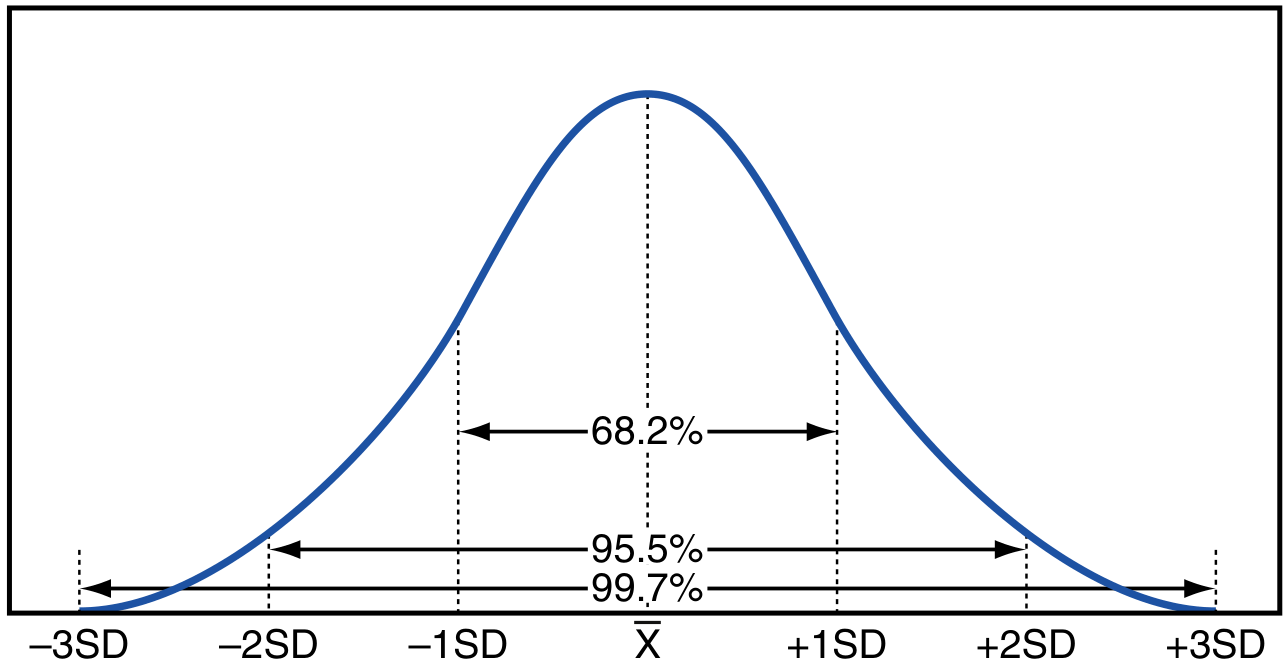
In a Normal (Gaussian) Distribution
From Quick Compendium of Clinical Pathology:
"In a perfect Gaussian distribution, mean, median, and mode are identical."
$$\text{Mean} = \text{Median} = \text{Mode}$$
In a Positively Skewed Distribution (Skewed Right)
The tail is on the right side. A few very high values pull the mean upward.
$$\text{Mode} < \text{Median} < \text{Mean}$$
Medical example: Income distribution, hospital waiting times, serum creatinine in a general population (most people have normal creatinine; a few have very high values due to renal failure).
In a Negatively Skewed Distribution (Skewed Left)
The tail is on the left side. A few very low values pull the mean downward.
$$\text{Mean} < \text{Median} < \text{Mode}$$
Medical example: Age at death in a developed country (most people die old; a few die young, pulling the mean down slightly).
Summary Table
| Distribution | Relationship |
|---|---|
| Normal (Gaussian) | Mean = Median = Mode |
| Positively skewed | Mode < Median < Mean |
| Negatively skewed | Mean < Median < Mode |
From Quick Compendium of Clinical Pathology:
"Some datasets are non-Gaussian - skewed positively or negatively. Skews alter the mean and median but do not affect the mode. In a positively skewed set of data, mean > median > mode."
6. The Geometric Mean
Definition
The geometric mean is the nth root of the product of n values. It is used when data spans several orders of magnitude or follows a log-normal distribution.
From Henry's Clinical Diagnosis:
"The geometric mean is calculated as the nth root of the product of a distribution of n numbers; its use for estimating central tendency minimizes the effects from extreme values such as are found in a log-normal distribution."
Formula
$$\text{Geometric Mean} = \sqrt[n]{x_1 \times x_2 \times \cdots \times x_n}$$
Or equivalently:
$$\log(\text{GM}) = \frac{\sum \log x_i}{n}$$
Medical Application
- Antibody titres (e.g., HBsAb levels after vaccination)
- Bacterial colony counts
- Drug concentration data (pharmacokinetics)
Example from the textbook:
Values: 3, 3, 4, 4, 5, 5, 5, 6, 6, 8, 9, 10, 15, 21
- Arithmetic mean = 7.2
- Geometric mean = 6.09 (better reflects the preponderance of lower values)
7. Which Measure to Use? (Decision Guide)
| Data Type | Distribution | Best Measure |
|---|---|---|
| Continuous | Normal (symmetric) | Mean |
| Continuous | Skewed / outliers present | Median |
| Categorical (nominal) | Any | Mode |
| Ordinal (ranked) | Any | Median |
| Log-normal (titres, counts) | Any | Geometric Mean |
| Bimodal population | Two peaks | Mode (both modes) |
From Cummings Otolaryngology:
"When SD is very large (larger than the mean value), the data often have an asymmetric distribution and should be described by the median and interquartile range. When in doubt, the median should always be used over the mean."
8. Worked Comprehensive Medical Example
Scenario: A physician records the systolic blood pressure (mmHg) of 10 patients in a hypertension clinic:
Values: 130, 145, 120, 160, 135, 145, 118, 150, 145, 132
Step 1 - Sort: 118, 120, 130, 132, 135, 145, 145, 145, 150, 160
Mean:
$$\bar{x} = \frac{118+120+130+132+135+145+145+145+150+160}{10} = \frac{1380}{10} = \textbf{138 mmHg}$$
Median: n = 10 (even) → Average of 5th and 6th values
$$= \frac{135 + 145}{2} = \textbf{140 mmHg}$$
Mode: 145 appears 3 times → Mode = 145 mmHg
Interpretation:
- Mean (138) < Median (140) < Mode (145)
- This suggests a slightly negatively skewed distribution
- The median (140 mmHg) is the best representative value for this skewed data
- The mode (145 mmHg) is the most common blood pressure recorded
9. Clinical Significance of Choosing the Right Measure
| Wrong choice | Consequence |
|---|---|
| Using mean in skewed income data | Overestimates typical household income |
| Using mean with one outlier (e.g., one patient with SBP 220) | Falsely elevates the "average" BP |
| Using mode for continuous data | Gives only one arbitrarily common value, not representative |
| Using median when data is truly normal | Wastes statistical power (mean would be better) |
10. Summary Table
| Feature | Mean | Median | Mode |
|---|---|---|---|
| Definition | Sum / n | Middle value | Most frequent |
| Formula | Σx/n | Positional | Count frequencies |
| Uses all values? | ✅ Yes | ❌ No | ❌ No |
| Affected by outliers? | ✅ Yes | ❌ No | ❌ No |
| Data type | Continuous | Continuous/Ordinal | Any (best for nominal) |
| Best distribution | Normal | Skewed | Categorical/Bimodal |
| Further calculations | ✅ Yes | ❌ Limited | ❌ No |
| In normal distribution | = Median = Mode | = Mean = Mode | = Mean = Median |
Conclusion
Measures of central tendency allow a researcher to represent an entire dataset with a single, meaningful value. The mean is the most powerful but sensitive to outliers. The median is the most reliable for real-world clinical data which is often skewed. The mode is the only measure usable for categorical data. Selecting the correct measure is not merely academic - it directly impacts clinical interpretation. A wrong choice can mislead clinical decisions, distort research conclusions, and misrepresent patient populations.
References:
- Quick Compendium of Clinical Pathology, 5th ed. - Section 8.3.1.1
- Henry's Clinical Diagnosis and Management by Laboratory Methods - Central Tendency & Statistics
- Swanson's Family Medicine Review - Biostatistics chapter
- Rockwood and Green's Fractures in Adults, 10th ed. - Descriptive Statistics
This is a shared conversation. Sign in to Orris to start your own chat.