Ct calcium scoring in detail, definition, principle , technique, equipment required, protocol , and all steps in detail
CT calcium scoring coronary artery calcification technique
CT Calcium Scoring (Coronary Artery Calcium Scoring — CAC)
1. Definition
"Coronary calcium is an indicator of the burden of atherosclerotic plaque, although there is no correlation of the amount of local coronary calcium with the physiologic or anatomic significance of an underlying coronary stenosis." — Goldman-Cecil Medicine
2. Principle
Pathophysiological Basis
- Calcification in the coronary arteries occurs almost exclusively in the setting of coronary atherosclerosis (with the exception of advanced chronic kidney disease).
- As the amount of coronary calcium roughly correlates to the extent of atherosclerotic plaque, its detection and quantification allows risk stratification.
- Most patients with acute coronary syndrome (ACS) have coronary calcium, and their calcium burden is substantially greater than in age- and sex-matched controls without CAD.
- Importantly, coronary calcification is not related to plaque stability/instability and is only weakly related to the severity of luminal stenosis — i.e., a heavily calcified plaque may not be obstructive.
Physical Principle
- CT acquires images by passing a thin X-ray beam through the body at multiple angles. X-ray transmission measurements are digitized into pixels — each assigned a value in Hounsfield units (HU), referenced to water (0 HU).
- Calcium is highly attenuating and appears bright white on non-contrast CT, even without contrast enhancement.
- A coronary lesion is defined as calcium when CT density is ≥ 130 HU with an area of ≥ 1 mm².
Agatston Score Calculation
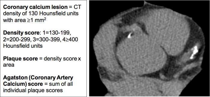
| HU Range | Density Weight Factor |
|---|---|
| 130–199 HU | 1 |
| 200–299 HU | 2 |
| 300–399 HU | 3 |
| ≥ 400 HU | 4 |
- The Agatston score corresponds to each coronary lesion's calcium area multiplied by the maximal CT attenuation value, then summed for the entire coronary tree.
- Less commonly, volume score (mm³) and calcium mass score (mg) are also used.
3. Score Interpretation / Categories
| Agatston Score | Category | Interpretation |
|---|---|---|
| 0 | Absent | No detectable calcification; very low risk |
| 1–10 | Minimal | Trace calcification |
| 10–100 | Mild | Mild plaque burden |
| 100–400 | Moderate | Moderate plaque burden |
| > 400 | Severe | Extensive plaque; high cardiovascular risk |
- Scores are age, sex, and race dependent; they are normalized and reported as percentile scores against population databases.
- Overall 15-year mortality rates in asymptomatic patients range from 3 to 28% for CAC scores from 0 to ≥ 1000.
- A CAC score of 0 (zero) is associated with excellent prognosis; future cardiac events are highly unlikely.
- CAC adds prognostic information independently of standard risk factors (Framingham risk score).
4. Equipment Required
CT Scanner
- Multi-detector CT (MDCT) scanner — the standard platform today
- Minimum: 16-slice MDCT; optimal: 64-slice or higher
- Modern scanners: 128–640 slice systems (dual-source CT, wide-detector CT)
- Electron Beam CT (EBCT) — the original scanner used for CAC scoring (now largely replaced by MDCT)
- Advantages of EBCT: very fast acquisition, less cardiac motion artefact
- Disadvantage: less widely available
ECG Synchronization
- ECG gating hardware — mandatory for cardiac motion suppression
- Prospective ECG triggering is standard for CAC scoring (triggers acquisition at a fixed phase of the cardiac cycle, typically mid-diastole)
- Reduces motion blur, minimises radiation dose
Other Required Equipment
- ECG electrodes and monitoring leads (3 or 4 lead setup)
- Cardiac calcium scoring post-processing software (e.g., Syngo.via [Siemens], AW workstation [GE], Extended Brilliance Workspace [Philips])
- Software automatically identifies lesions ≥ 130 HU and calculates per-vessel and total Agatston scores with color-coded overlays
5. Indications
- Asymptomatic adults at intermediate cardiovascular risk (10–20% 10-year event risk) — most validated indication, can "upgrade" or "downgrade" risk category
- Asymptomatic patients at low risk with a family history of premature ischaemic heart disease
- Patients where statin therapy decision is uncertain after clinical risk assessment
- Not indicated in symptomatic patients (a negative CAC score does not exclude obstructive CAD in young or symptomatic patients)
6. Contraindications / Limitations
- Symptomatic patients — a zero CAC score does not reliably exclude CAD (especially in young patients with non-calcified soft plaques)
- Patients with known CAD or prior revascularisation — rarely changes management
- Already low-risk or already high-risk patients — adds limited incremental value (a very high CAC may prompt stress testing)
- Pregnancy — ionising radiation contraindicated
- Advanced CKD — calcification may occur without atherosclerosis, reducing specificity
- Irregular heart rhythm (AF) — impairs ECG gating, though modern software can compensate
7. Patient Preparation
- No iodinated contrast is required — this is a plain (non-contrast) scan
- Patient should avoid caffeine and smoking for several hours before the scan (may affect heart rate)
- Ideally, heart rate should be below 65–70 bpm for adequate gating, though CAC is more forgiving than CTA
- Beta-blockers may be given to lower heart rate if needed (more critical for CT angiography)
- Explain the procedure; no special fasting required (unlike contrast studies)
- Remove metallic objects from the chest area
- Attach ECG electrodes to the chest
8. Scan Protocol — Step by Step
Step 1: Scout / Topogram
- Acquire a low-dose AP scout image of the chest
- Used to define the scan range: from the carina (level of the tracheal bifurcation) down to the diaphragm, encompassing the entire heart
Step 2: ECG Electrode Placement and Monitoring
- Attach 3–4 lead ECG electrodes to the patient's chest
- Verify a clean ECG signal on the console
- Prospective ECG triggering: acquisition is triggered at ~70–75% of the R–R interval (mid-diastole), when the heart is most still
Step 3: Breath-Hold Instruction
- Instruct the patient to take a moderate breath-hold (not a forced deep inspiration) during acquisition
- Typically 10–15 seconds
Step 4: Acquisition Parameters
| Parameter | Typical Value |
|---|---|
| Tube voltage (kVp) | 120 kVp (standard); 100 kVp for smaller patients |
| Tube current (mAs) | 50–100 mAs (low dose) |
| Slice thickness | 2.5–3 mm (standard for Agatston); reconstructed at 2.5 mm |
| Rotation time | 0.35–0.5 sec |
| Gating mode | Prospective ECG triggering |
| Reconstruction kernel | Medium-smooth (e.g., B35f or similar) |
| Field of view (FOV) | Heart-centred, ~25 cm |
| Matrix | 512 × 512 |
| Scan direction | Cranio-caudal |
Note: Slice thickness of 2.5–3 mm is standardised for Agatston scoring; thinner slices (used in CT angiography) do not yield directly comparable Agatston scores.
Step 5: Radiation Dose
- Radiation dose is intentionally very low: approximately 1–2 mSv (comparable to a few months of background radiation)
- Prospective gating significantly reduces dose compared to retrospective spiral acquisition
9. Image Reconstruction and Post-Processing
Step 1: Reconstruction
- Images are reconstructed at 2.5 mm slice thickness with a medium-smooth kernel
- Iterative reconstruction algorithms (e.g., SAFIRE, iDose, ASIR) reduce image noise — allow diagnostic quality even at low dose
Step 2: Transfer to Calcium Scoring Workstation
- DICOM images are sent to dedicated cardiac scoring software
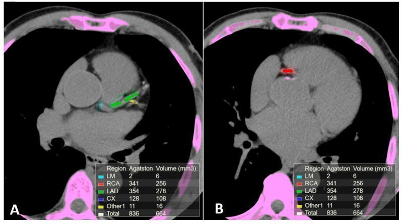
Step 3: Automated Lesion Detection
- Software automatically identifies all foci ≥ 130 HU with area ≥ 1 mm²
- Highlights them with color-coded overlays by coronary territory (e.g., LM = cyan, LAD = green, RCA = red, LCx = blue)
- Assigns density weight factors (1–4) based on peak HU
Step 4: Manual Review and Editing
- The radiologist/technologist reviews each detected lesion
- False positives must be excluded: papillary muscle calcification, mitral/aortic valve calcifications, sternal wires, pericardial calcification — these are NOT coronary and must be deleted from the ROI
- False negatives from automated algorithms can occur in extensive calcification
Step 5: Per-Vessel Score Reporting
- Scores are reported per vessel (LM, LAD, LCx, RCA) and as a total
- Volume (mm³) is also calculated as a secondary metric
- Total score is compared to age/sex/race-matched percentile tables and the patient is placed in a risk percentile
10. CT Images — Grades of CAC

11. Reporting
- Total Agatston score
- Per-vessel Agatston scores (LM, LAD, LCx, RCA)
- Volume score (total, mm³)
- Age/sex/race-adjusted percentile
- Risk category (absent / minimal / mild / moderate / severe)
- Incidental findings on the scan (lung nodules, pleural effusion, aortic aneurysm, etc.) — important added value of every CAC scan
- Clinical correlation and recommendation (e.g., discuss with clinician regarding statin initiation)
12. Clinical Utility
- Primary prevention risk stratification: CAC is currently the strongest imaging-based predictor of future MI and cardiac death in asymptomatic patients
- Useful to reclassify intermediate-risk patients — a zero score may defer statin therapy; a high score may escalate it
- High scores may prompt stress testing even in otherwise low-symptom patients
- CAC can also be acquired as a by-product during hybrid SPECT/CT or PET/CT scans
- CAC scoring does not require contrast, making it suitable for patients with renal insufficiency or contrast allergy when coronary CTA would be contraindicated
13. Radiation Dose Comparison
| Examination | Approximate Dose |
|---|---|
| CAC scoring | 1–2 mSv |
| Coronary CT angiography | 3–15 mSv |
| Standard chest X-ray | 0.05–0.1 mSv |
| Annual background radiation | ~2.4 mSv |
Summary
| Feature | Detail |
|---|---|
| Scan type | Non-contrast, ECG-gated CT |
| Contrast | None required |
| Target | Coronary artery calcification |
| Primary score | Agatston score |
| Threshold | ≥ 130 HU, ≥ 1 mm² |
| Slice thickness | 2.5–3 mm |
| Radiation dose | ~1–2 mSv |
| Main indication | Intermediate-risk asymptomatic adults |
| Key limitation | Does not assess non-calcified (soft) plaque |
- Harrison's Principles of Internal Medicine, 22nd Ed. (2025), Ch. 248 & 284
- Goldman-Cecil Medicine, International Ed., Ch. 44
- Grainger & Allison's Diagnostic Radiology, Ch. 15
- Fuster and Hurst's The Heart, 15th Ed., Ch. 21
Now ct perfusion scanning in detail as u give above , and also add diagram that I can draw in exam
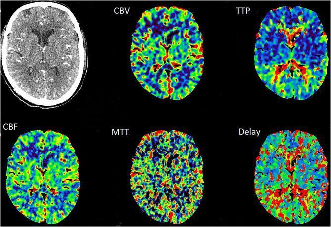
CT perfusion brain cerebral blood flow CBF CBV MTT map
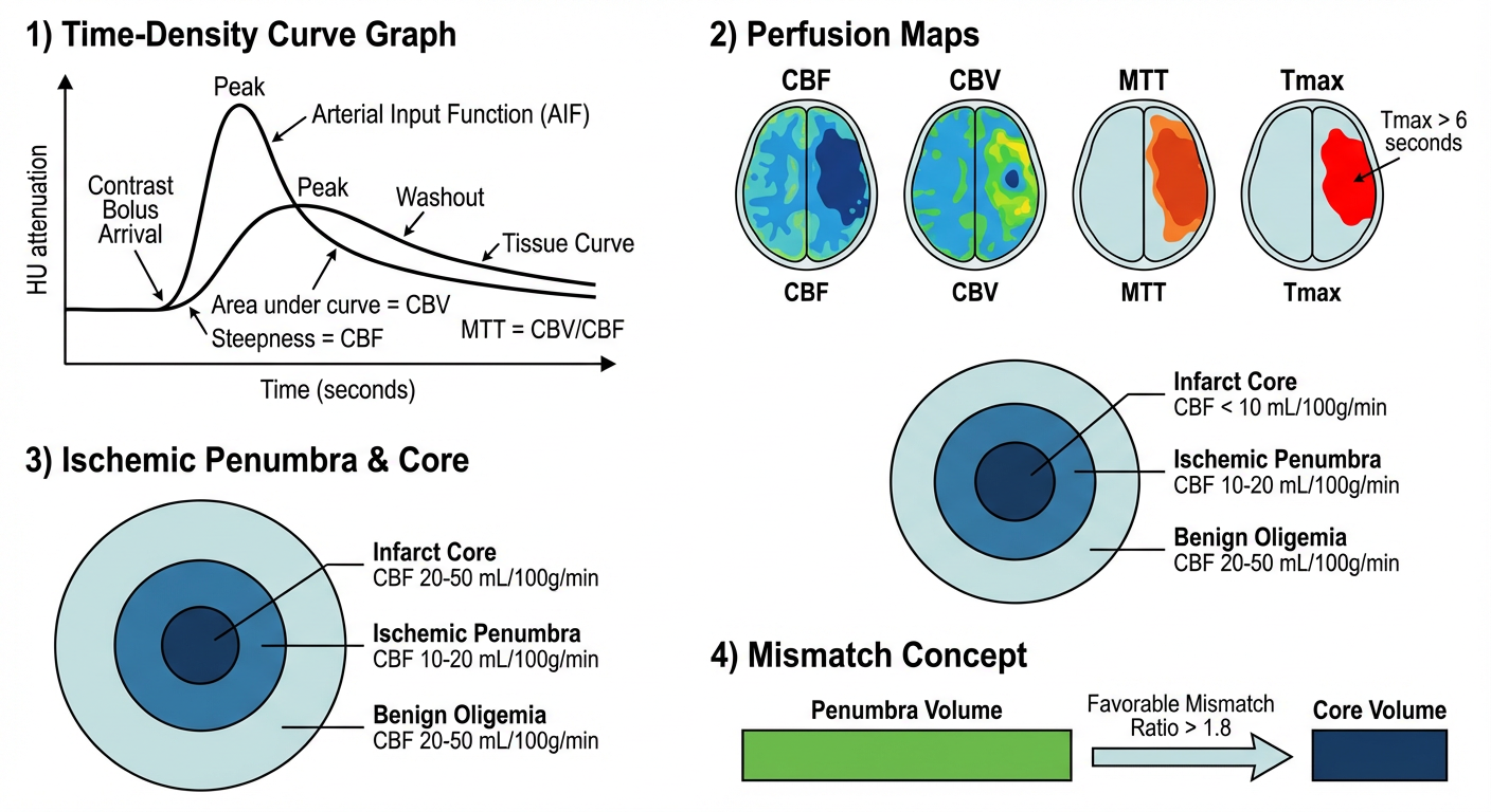
A clean educational medical diagram for exam use showing CT perfusion brain scanning workflow. The diagram has four sections arranged top to bottom: 1) Time-density curve graph showing arterial input function (AIF) and tissue curve with contrast bolus arrival, peak, and washout phases on x-axis (time in seconds) and y-axis (HU attenuation). Key areas labeled: area under curve = CBV, steepness = CBF, MTT = CBV/CBF. 2) Four color-coded perfusion maps side by side labeled CBF, CBV, MTT, Tmax - each showing a simplified brain axial outline with an ischemic region. CBF shows dark blue deficit area, CBV shows preserved volume in penumbra, MTT shows prolonged red-orange region, Tmax greater than 6 seconds highlighted. 3) A concentric circle diagram showing infarct core (center, darkest) surrounded by ischemic penumbra, surrounded by benign oligemia - with CBF values labeled: core less than 10 mL/100g/min, penumbra 10-20 mL/100g/min, oligemia 20-50 mL/100g/min. 4) Mismatch concept: two bars comparing penumbra volume vs core volume, showing favorable mismatch ratio greater than 1.8. All text labels in black, clean white background, suitable for hand-drawing reference in medical exams.
CT Perfusion Scanning (CTP) — In Detail
1. Definition
"CT perfusion scans generate quantitative color maps that indicate various physiologic parameters such as cerebral blood flow (CBF), cerebral blood volume (CBV), and mean transit time (MTT) through quantitative analysis of rapidly acquired image sequences during intravenous contrast administration." — Schwartz's Principles of Surgery
2. Principle
Physiological Basis
- Vasodilation → increases CBV, maintains CBF
- Blood cells spend longer in the tissue → MTT prolongs
- If vessels are maximally dilated and CPP drops further → CBF falls
- Oxygen extraction increases maximally, then cellular dysfunction begins
- When CBF < 15–20 mL/100g/min → loss of electrical neuronal function
- When CBF < 10 mL/100g/min → ATP failure → Na⁺/K⁺ pump failure → cytotoxic oedema → irreversible infarction
The Penumbra Model
| Zone | CBF | Cell Status |
|---|---|---|
| Infarct core | < 10 mL/100g/min | Dead — irreversible |
| Ischaemic penumbra | 10–20 mL/100g/min | Alive but dysfunctional — salvageable |
| Benign oligaemia | 20–50 mL/100g/min | Mildly reduced — will survive |
Physical / Mathematical Principle
- A bolus of iodinated contrast is injected IV
- The contrast transiently increases CT attenuation (HU) as it passes through tissue
- Repeated CT acquisitions are made rapidly over the same slices — generating a time-density curve (TDC) at every pixel
- Two curves are generated: the arterial input function (AIF) from a large artery, and the tissue curve from brain parenchyma
| Parameter | Derived From | Represents |
|---|---|---|
| CBV | Area under the tissue curve (relative to AIF) | Volume of blood per 100g tissue (mL/100g) |
| CBF | Gradient / peak of deconvolved residue function | Flow of blood per 100g tissue per minute (mL/100g/min) |
| MTT | Central volume principle: MTT = CBV ÷ CBF | Average transit time of blood through tissue (seconds) |
| Tmax | Time to maximum of residue function | Delay between AIF and tissue bolus arrival — best marker of penumbra |
| TTP | Time from injection to peak enhancement | Simpler, no AIF deconvolution needed |
3. Key Parameters — Normal Values and Significance
| Parameter | Normal Value | In Penumbra | In Core Infarct |
|---|---|---|---|
| CBF | 50–55 mL/100g/min | ↓ (10–20) | ↓↓ (< 10) |
| CBV | 4–6 mL/100g | Preserved or ↑ | ↓ (microvascular collapse) |
| MTT | 4–6 seconds | Prolonged ↑ | Very prolonged |
| Tmax | < 6 seconds | > 6 s (penumbra threshold) | > 10 s |
| TTP | Short | Delayed | Very delayed |
- Core = CBF severely reduced AND CBV reduced (microvascular collapse)
- Penumbra = CBF moderately reduced BUT CBV preserved (autoregulation still working)
- Mismatch = Penumbra volume ≥ 20% larger than core → favourable for reperfusion therapy
4. Exam Diagram
How to Draw in Exam — Step by Step
HU
↑        AIF (tall, sharp peak)
|       /\
|      /  \      Tissue curve (low, broad)
|    /    \   /‾‾‾\
|  /      \_/      \___
+________________________→ Time (sec)

Area under tissue curve = CBV
Peak height / steepness = related to CBF
MTT = CBV ÷ CBF
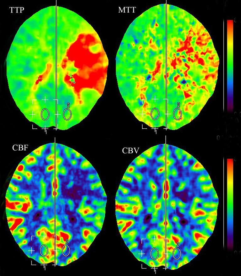
- CBF → dark hole on one side (reduced)
- CBV → smaller hole (core only reduced; penumbra preserved)
- MTT → large bright/prolonged area
- Tmax → largest area of delay (>6s = penumbra threshold)
         Benign oligaemia (CBF 20-50)
       ┌──────────────────────────┐
       │   Ischaemic penumbra     │
       │    ┌──────────────┐      │
       │    │  INFARCT     │      │
       │    │    CORE      │      │
       │    │ CBF < 10     │      │
       │    └──────────────┘      │
       │     CBF 10–20            │
       └──────────────────────────┘
              CBF 20–50
|████████████████████████| ← Penumbra volume
|████████|                ← Core volume
         ↑
    Mismatch ratio ≥ 1.8 → TREAT (thrombectomy/thrombolysis)
5. CTP Perfusion Maps — Clinical Images
6. Equipment Required
CT Scanner
- Multi-detector CT (MDCT) — minimum 64-slice; optimal 128-slice or higher
- Wide-detector CT (256–320 slice) — covers the entire brain in a single rotation without table movement; reduces radiation and motion artefact (preferred)
- Older systems required toggling (shuttling) the table back and forth to cover the whole brain
- Modern photon-counting CT — improved resolution and reduced dose
Contrast Injector
- Dual-head power injector — delivers contrast at precise rate (typically 4–6 mL/sec) followed by saline flush
- Required for tight, reproducible bolus
Monitoring
- ECG monitoring (not mandatory but useful if arrhythmia suspected)
- Pulse oximetry and IV access
Post-Processing Software
- Dedicated perfusion workstation software (e.g., Syngo.via [Siemens], IntelliSpace [Philips], Advantage Workstation [GE], RAPID [iSchemaView] — the most validated for stroke)
- Software performs:
- Automated AIF selection
- Deconvolution algorithms
- Colour map generation
- Core vs. penumbra segmentation
- Mismatch ratio calculation
7. Indications
Neurological (Primary — Brain CTP)
- Acute ischaemic stroke — most important indication
- Identify ischaemic core vs. salvageable penumbra
- Guide decision for IV thrombolysis (tPA) and mechanical thrombectomy
- Extended time window (6–24 hours) — patient selection by DAWN/DEFUSE-3 criteria
- Transient ischaemic attack (TIA) — detect occult hypoperfusion
- Vasospasm after subarachnoid haemorrhage — assess delayed cerebral ischaemia
- Brain tumours — assess vascularity, grade, distinguish recurrence from radiation necrosis
- Pre-surgical cerebrovascular reserve assessment
Non-Neurological Uses
- Acute pancreatitis — detect pancreatic necrosis earlier than conventional CT
- Oncology — assess tumour perfusion, angiogenesis, treatment response (lung, liver, pancreas)
- Pulmonary nodules — differentiate malignant from benign
8. Patient Preparation
- IV access — large-bore antecubital vein (18G or larger), right arm preferred (avoids left brachiocephalic vein artefact on CTA)
- Assess renal function — eGFR > 30 mL/min/1.73m² preferred; in acute stroke, benefit usually outweighs risk
- Contrast allergy history — premedication if previous mild reaction; avoid if severe prior anaphylaxis
- Metformin — hold for 48 hours after contrast if eGFR < 60
- Establish IV line patency — extravasation must be avoided (high injection rate)
- Explain procedure — reassure regarding warmth/flushing sensation from contrast
- Patient lies supine and still — head in headrest/immobiliser
- No breath-hold required (unlike cardiac CT) — the brain does not move with breathing
9. Scan Protocol — Step by Step
Step 1: Non-Contrast CT (NECT)
- Standard axial NECT of the brain first — mandatory
- Purpose: exclude haemorrhage before contrast, assess ASPECTS score, identify hyperdense vessel sign
- Parameters: 120 kVp, standard dose, 5mm slices, brain/bone window
Step 2: CT Angiography (CTA)
- Performed as part of multimodal CT in most acute stroke protocols
- Contrast bolus (60–80 mL at 4–5 mL/sec) with bolus tracking trigger on aortic arch
- Covers arch of aorta to vertex — assesses for large vessel occlusion (LVO)
Step 3: CT Perfusion Acquisition
| Parameter | Value |
|---|---|
| Contrast volume | 40–50 mL |
| Injection rate | 4–6 mL/sec |
| Saline flush | 30–40 mL at same rate |
| Contrast concentration | 300–400 mgI/mL |
| Parameter | Value |
|---|---|
| Scan delay | 4–6 seconds post-injection start |
| Scan duration | 40–60 seconds of dynamic acquisition |
| Tube voltage | 80–100 kVp (lower = better iodine contrast) |
| Tube current | 100–200 mA (low dose) |
| Rotation time | 0.5 sec |
| Slice thickness | 5–10 mm (brain CTP) |
| Coverage | 80–160 mm (wide-detector CT: whole brain) |
| Mode | Toggling or fixed-table depending on scanner |
| Frame rate | 1 image/second per location |
Step 4: Image Acquisition Sequence
Inject contrast IV (4-6 mL/sec)
        ↓
Start CT acquisition at 4-6 sec delay
        ↓
Repeated CT passes over same brain levels
  → every 1-2 seconds for 40-60 seconds
        ↓
Generates ~40-60 time-points per level
        ↓
Time-density curve built for every pixel
Step 5: Post-Processing
- Motion correction — automated realignment of all time-point images
- Vessel identification — AIF selected (usually MCA or ACA), venous output function (VOF) selected from superior sagittal sinus
- Deconvolution — mathematical calculation of CBF, CBV, MTT, Tmax for every pixel
- Threshold application — software applies validated thresholds:
- Core: CBF < 30% of contralateral (or CBF < 10 mL/100g/min)
- Penumbra: Tmax > 6 seconds
- Colour map generation — colour-coded parametric maps displayed
- Mismatch calculation — penumbra volume ÷ core volume → mismatch ratio
Step 6: Reporting
- Core infarct volume (mL)
- Penumbra volume (mL)
- Mismatch ratio and mismatch volume
- Presence/absence of large vessel occlusion (from CTA)
- Any haemorrhagic transformation
- Collateral flow assessment
10. Stroke Treatment Criteria Using CTP (DAWN / DEFUSE-3)
| Criteria | Value |
|---|---|
| Core infarct volume (6–16 hr) | ≤ 70 mL |
| Core-penumbra mismatch volume | ≥ 15 mL |
| Mismatch ratio | ≥ 1.8 |
| Tmax threshold for penumbra | > 6 seconds |
| Core infarct (16–24 hr) | ≤ 70 mL (DAWN) |
"CT perfusion within 6–16 hr: core infarct volume ≤70 mL, core-penumbra mismatch volume ≥15 mL, core-penumbra mismatch ratio ≥1.8" — Washington Manual of Medical Therapeutics
11. Radiation Dose
| Component | Approximate Dose |
|---|---|
| NECT brain | 1–2 mSv |
| CTP alone | 3–8 mSv |
| Full multimodal CT (NECT + CTA + CTP) | 5–12 mSv |
12. Limitations and Pitfalls
| Limitation | Detail |
|---|---|
| Motion artefact | Patient head movement degrades maps — motion correction algorithms partially compensate |
| AIF selection error | Incorrect AIF placement leads to systematic errors in all maps |
| Limited brain coverage (older scanners) | Toggling misses the full brain; wide-detector CT solves this |
| Contrast contraindications | Renal failure, allergy |
| Tmax sensitivity to AIF | Small AIF shape variations alter Tmax maps significantly |
| Does not show non-perfusion causes | Metabolic, toxic, or ictal causes of deficits may mimic perfusion abnormality |
| Threshold variability | Different platforms use different CBF/CBV thresholds — limit inter-institution comparison |
| Not for haemorrhagic stroke | Contrast contraindicated in active large haemorrhage |
13. Comparison of CT Perfusion vs. MR Perfusion
| Feature | CTP | MR Perfusion (PWI) |
|---|---|---|
| Speed | Fast (~1 min) | Slower |
| Availability | Widely available | Less available acutely |
| Radiation | Yes (3–8 mSv) | No |
| Contrast | Iodinated | Gadolinium |
| Sensitivity to haemorrhage | Good (NECT done first) | Better (SWI/GRE) |
| Motion artefact | Less susceptible | More susceptible |
| Spatial resolution | Slightly lower | Higher |
| Core marker | CBF < 30% or CBV reduced | DWI |
| Penumbra marker | Tmax > 6 sec | Tmax > 6 sec (PWI) |
14. Summary Table
| Feature | Detail |
|---|---|
| Scan type | Dynamic contrast-enhanced CT |
| Contrast | Iodinated IV, 40–50 mL at 4–6 mL/sec |
| Duration of dynamic scan | 40–60 seconds |
| Primary maps | CBF, CBV, MTT, Tmax |
| Core threshold | Tmax > 10s or CBF < 30% contralateral |
| Penumbra threshold | Tmax > 6 seconds |
| Mismatch for treatment | Ratio ≥ 1.8, volume ≥ 15 mL |
| Main clinical indication | Acute ischaemic stroke |
| Radiation dose | 3–8 mSv |
| Key formula | MTT = CBV ÷ CBF |
- Grainger & Allison's Diagnostic Radiology, Ch. 56 (Acute Stroke Imaging)
- Harrison's Principles of Internal Medicine, 22nd Ed., Ch. 434
- Schwartz's Principles of Surgery, 11th Ed., Ch. 42
- Washington Manual of Medical Therapeutics
- Rosen's Emergency Medicine, Ch. 14
Myocardial imaging in detail in ct ?
myocardial CT imaging cardiac perfusion late enhancement viability
cardiac CT myocardial perfusion stress adenosine short axis LV defect
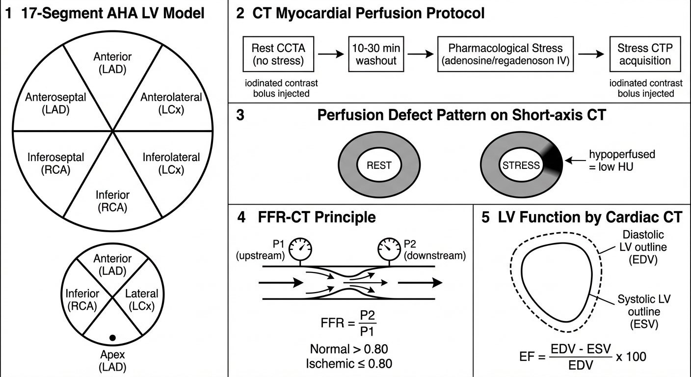
A clean, labeled educational medical exam diagram showing myocardial CT imaging. The diagram is divided into 5 clearly labeled sections arranged vertically on white background with black text: Section 1 - "17-Segment AHA LV Model": draw a short-axis circle (the left ventricle) divided into 6 segments labeled anterior, anteroseptal, inferoseptal, inferior, inferolateral, anterolateral, with a small apical circle below showing 4 segments, and an apex point. Each segment labeled with coronary territory (LAD, RCA, LCx). Section 2 - "CT Myocardial Perfusion Protocol": a horizontal flowchart showing: Rest CCTA (no stress) arrow to 10-30 min washout arrow to Pharmacological Stress (adenosine/regadenoson IV) arrow to Stress CTP acquisition, with iodinated contrast bolus injected during each phase. Section 3 - "Perfusion Defect Pattern on Short-axis CT": draw two side-by-side short-axis LV circles. Left labeled REST - uniform grey myocardium. Right labeled STRESS - dark wedge-shaped hypoattenuation defect in anteroseptal wall. Arrow pointing to defect saying "hypoperfused = low HU". Section 4 - "FFR-CT Principle": draw a coronary artery with a stenosis, then computational fluid dynamics arrows, showing pressure drop P1 upstream and P2 downstream, FFR = P2/P1, normal greater than 0.80, ischemic less than or equal to 0.80. Section 5 - "LV Function by Cardiac CT": diastolic LV outline (larger) and systolic LV outline (smaller) overlaid, with formula EF = EDV minus ESV divided by EDV x 100. Clean labels, no color fills, line-art suitable for exam hand-drawing.
Myocardial Imaging in CT — In Detail
1. Overview and Definition
- Morphology and structure — wall thickness, mass, volume
- Global and regional systolic function — ejection fraction, wall motion
- Myocardial perfusion — stress CT perfusion (CTP), detection of ischaemia
- Myocardial viability and tissue characterisation — infarct, fibrosis, oedema
- Physiological significance of stenosis — CT-derived FFR (FFR-CT)
"Stress CT myocardial perfusion may be used for evaluating myocardial perfusion for the detection of functionally significant coronary artery disease." — Grainger & Allison's Diagnostic Radiology
"Evolving new applications for the adjudication of the hemodynamic significance of stenosis such as CT myocardial perfusion imaging and FFR-CT are now being used in clinical practice." — Fuster and Hurst's The Heart, 15th Ed.
2. Why CT for Myocardial Imaging?
- Excellent spatial resolution (< 0.5 mm in-plane) — superior to nuclear or echo
- True 3D volumetric dataset — any plane can be reconstructed
- Fast acquisition — full heart in 5–15 seconds
- Ability to combine anatomy (CCTA) + perfusion (CTP) + function in a single session
- Limitation: ionising radiation, iodinated contrast, heart rate dependency
3. Exam Diagram
MODULE A: CT Assessment of Ventricular Morphology and Function
3A.1 Acquisition Requirements
- ECG-gated MDCT — mandatory to freeze cardiac motion
- Two acquisition modes:
| Mode | Description | Use |
|---|---|---|
| Prospective ECG triggering | Images acquired at one fixed phase (~75% R-R, mid-diastole) | Coronary anatomy; low dose ~2–5 mSv |
| Retrospective ECG gating | Continuous helical acquisition throughout entire cardiac cycle; any phase reconstructable | Ventricular function, wall motion; higher dose 12–21 mSv; dose modulation reduces this |
- For LV function alone: low-dose cine CT throughout cardiac cycle suffices
- Iodinated contrast is required (except for CAC scoring)
3A.2 Standard Reconstructed Views
Short-axis views (basal, mid, apical):
Each ring divided into 6 (basal/mid) or 4 (apical) segments
+ Apex = segment 17

Coronary territory assignment:
  LAD  → anterior, anteroseptal, apical segments
  RCA  → inferior, inferoseptal segments
  LCx  → lateral, inferolateral segments
- Short-axis (SA) — most important; perpendicular to LV long axis
- Two-chamber (vertical long axis)
- Four-chamber (horizontal long axis)
- Three-chamber (LV outflow tract view)
3A.3 Ventricular Volume and Ejection Fraction
- End-diastolic volume (EDV) and end-systolic volume (ESV) are measured from contoured endocardial borders
- EF = (EDV − ESV) ÷ EDV × 100
- CT is highly accurate for volumetric analysis — more so than 2D echo
- LV mass = (epicardial volume − endocardial volume) × myocardial density (1.05 g/mL)
3A.4 Regional Wall Motion Assessment
- From functional cine reconstruction, systolic wall thickening and inward endocardial motion are assessed per segment
- Wall motion abnormalities (hypokinesis, akinesis, dyskinesis) in a coronary distribution = ischaemic aetiology
- Ventricular thinning + wall motion abnormality = scar / prior MI
MODULE B: CT Myocardial Perfusion Imaging (CT-MPI / CTP)
3B.1 Principle
- A coronary stenosis may not limit blood flow at rest (autoregulation compensates)
- Pharmacological vasodilators (adenosine, dipyridamole, regadenoson) maximally dilate normal microvessels → increase flow in normal territories 3–5× above baseline
- Stenosed arteries cannot match this → relative hypoperfusion = perfusion defect appears on CT as hypoattenuation
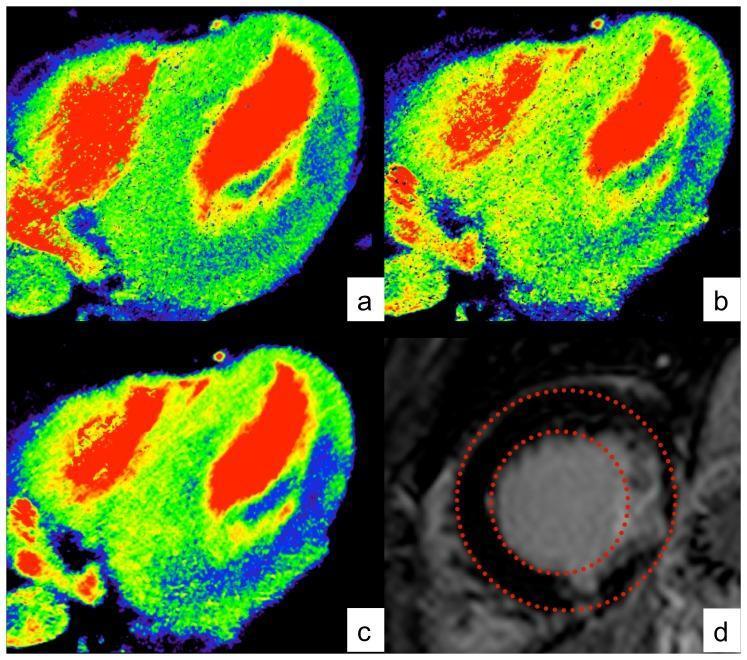
3B.2 Two Types of CT Perfusion
| Type | Description |
|---|---|
| Static CTP (single phase) | One image at peak contrast enhancement during stress → detects relative hypoattenuation; simpler, lower dose |
| Dynamic CTP | Serial CT acquisitions over time during contrast bolus → generates quantitative parametric maps of MBF (mL/min/g); similar to brain CTP |
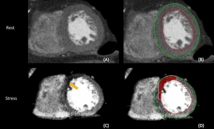
3B.3 Protocol
Step 1: Rest CCTA (coronary CT angiography)
           ↓
        10–30 minute washout interval
        (allow contrast to clear + vasodilator to wear off)
           ↓
Step 2: Pharmacological stress
        → Adenosine 140 µg/kg/min IV × 3 min, OR
        → Regadenoson 0.4 mg IV bolus
           ↓
Step 3: IV contrast (40–60 mL at 5 mL/sec) injected
           ↓
Step 4: Stress CTP acquisition during peak myocardial enhancement
        → Timed bolus tracking or fixed delay (~30 sec post-injection)
           ↓
Step 5: Post-processing — short-axis colour maps generated
        → Perfusion defect = dark area (↓ HU) during stress
        → Normal myocardium = bright (↑ HU)
3B.4 Acquisition Parameters for Stress CTP
| Parameter | Value |
|---|---|
| kVp | 80–100 kVp (lower = better iodine contrast) |
| mAs | 200–400 (higher than rest for SNR) |
| Gating | Prospective ECG triggering |
| Coverage | 80–160 mm (wide detector) or table toggle (older scanners) |
| Slice thickness | 0.6–1.5 mm reconstructed |
| Heart phase | End-diastole (~75% R-R) |
| Rotation time | 0.25–0.35 sec |
| Radiation dose | ~3–5 mSv (static); ~5–8 mSv (dynamic) |
3B.5 Image Interpretation
| Finding | Interpretation |
|---|---|
| Stress defect only (reversible) | Inducible ischaemia — viable but jeopardised myocardium |
| Stress + rest defect (fixed) | Prior MI / scar (non-viable) |
| No defect (normal) | No flow-limiting stenosis |
| Subendocardial defect | More common; subendocardium most vulnerable to ischaemia |
| Transmural defect | Full-thickness infarction |
MODULE C: FFR-CT (CT-Derived Fractional Flow Reserve)
3C.1 Definition and Principle
- Pa = aortic (coronary inlet) pressure
- Pd = distal coronary pressure beyond the stenosis
- Normal FFR = 1.0; haemodynamically significant stenosis = FFR ≤ 0.80
3C.2 How FFR-CT Works
Standard resting CCTA
         ↓
Coronary artery segmentation (automated)
         ↓
3D mesh model of coronary tree built
         ↓
Computational fluid dynamics applied:
  → Patient-specific microvascular resistance assigned
  → Hyperaemic conditions simulated mathematically
         ↓
Pressure gradient calculated at every point
         ↓
FFR displayed as colour map along coronary tree
  Red/orange = FFR ≤ 0.80 (ischaemia-causing)
  Green = FFR > 0.80 (non-significant)
3C.3 Performance Data
| Trial | Finding |
|---|---|
| DISCOVER-FLOW | FFR-CT more accurate than CTA alone for lesion-specific ischaemia |
| DeFACTO | Improved per-vessel diagnostic accuracy over CTA |
| NXT | Per-vessel accuracy: AUC 0.90 for FFR-CT vs 0.81 for CTA alone |
- Nonobstructive CAD found in only 12% of FFR-CT guided patients who proceeded to ICA vs 73% in standard care
- 61% of CCTA/FFR-CT patients had ICA cancelled with no adverse events
- Significantly less expensive and better QoL improvement
3C.4 When to Use FFR-CT
- Intermediate coronary stenosis on CCTA (40–70% stenosis) where functional significance is unclear
- Avoids need for invasive angiography or stress testing
- Particularly useful for 50–69% stenoses where CTA alone performs poorly
MODULE D: Myocardial Tissue Characterisation by CT
3D.1 CT Myocardial Infarction Detection
| Finding | CT Appearance | Significance |
|---|---|---|
| Acute MI | Hypoattenuation (dark) in myocardium during arterial phase | Reduced perfusion in infarcted zone |
| Chronic MI / Scar | Myocardial thinning (< 6 mm) + hypoattenuation | Full-thickness scar; non-viable |
| Microvascular obstruction | Persistent dark core after contrast — "no-reflow" | Worst prognosis after MI |
| Late iodine enhancement (LIE) | Hyperattenuation on 10-min delayed CT (analogous to LGE-CMR) | Extracellular iodine accumulation in fibrosis/scar |
- Iodinated contrast behaves similarly to gadolinium in infarcted tissue
- In scarred/fibrotic myocardium, extracellular space is expanded → contrast pools → delayed hyperattenuation on CT at 5–15 minutes post-injection
- Subendocardial LIE in a coronary distribution = ischaemic scar (analogous to LGE-CMR)
- Transmural LIE = extensive infarction
3D.2 CT Appearance of Myocardial Conditions
| Condition | CT Finding |
|---|---|
| Normal myocardium | Uniform 80–100 HU after contrast |
| Acute ischaemia / infarction | Subendocardial or transmural hypoattenuation (dark wedge) |
| Chronic MI / scar | Thinned wall (< 6 mm), hypoattenuation; ± LIE |
| LV aneurysm | Dyskinetic, thinned, bulging wall; ± thrombus (low HU) |
| Thrombus | Low HU (20–40 HU), non-enhancing filling defect |
| Hypertrophic cardiomyopathy (HCM) | Asymmetric LV hypertrophy; sigmoid septum; SAM |
| Dilated cardiomyopathy | Global LV dilatation, thin walls, reduced EF |
| Cardiac amyloid | Diffuse concentric thickening; subendocardial LIE |
| Myocarditis | Subepicardial/mid-wall LIE in non-coronary distribution |
| Pericardial effusion | Low-attenuation rim around heart; HU varies with content |
3D.3 Myocardial Fat
- Fat appears as very low HU (−50 to −100 HU) within myocardium
- Seen in: lipomatous metaplasia of old infarct, arrhythmogenic right ventricular cardiomyopathy (ARVC), cardiac lipoma
- ARVC: fatty replacement of RV free wall — CT highly sensitive
MODULE E: Cardiac CT for Structural Heart Disease
3E.1 Pre-TAVR CT Protocol
- Aortic annulus measurement — true short-axis plane, measured in systole
- Annular area, perimeter, short and long diameters
- Used for prosthetic valve sizing
- Aortic root anatomy — sinus of Valsalva dimensions, coronary ostia heights
- Left ventricular outflow tract (LVOT) assessment
- Iliofemoral access route assessment for catheter delivery
- Calcium scoring of aortic valve and LVOT
3E.2 Other Structural Uses
| Indication | CT Contribution |
|---|---|
| Pulmonary vein mapping (pre-AF ablation) | Pulmonary vein anatomy, ostial diameters |
| Left atrial appendage (LAA) thrombus | LAA filling defect (low HU) on CTA |
| Congenital heart disease | Anomalous vessels, septal defects, complex anatomy |
| Cardiac masses / tumours | Characterise location, density, vascularity, pericardial involvement |
| Pericardial disease | Thickness, calcification, effusion, constriction |
MODULE F: Comparison of Cardiac CT with Other Modalities
| Parameter | Cardiac CT | CMR (MRI) | Echocardiography | Nuclear (SPECT/PET) |
|---|---|---|---|---|
| Coronary anatomy | Excellent | Poor | Poor | None |
| LV volumes / EF | Excellent | Gold standard | Good | Good |
| Myocardial perfusion | Good (CTP) | Gold standard | Limited | Good |
| Tissue characterisation | Moderate (LIE) | Gold standard (LGE) | Poor | Moderate |
| Calcification | Excellent | Poor | Poor | None |
| Radiation | Yes (2–12 mSv) | None | None | Yes (5–15 mSv) |
| Claustrophobia | Rare issue | Major issue | None | Rare |
| Heart rate dependency | Yes | Less | No | No |
| Scan time | Minutes | 30–60 min | 20–30 min | 30–90 min |
MODULE G: Protocols Summary — Complete Cardiac CT Study
| Step | Scan | Purpose | Contrast |
|---|---|---|---|
| 1 | CAC scoring | Cardiovascular risk | None |
| 2 | Rest CCTA | Coronary anatomy, plaque | Yes |
| 3 | FFR-CT (post-processing) | Haemodynamic significance | Same images |
| 4 | Stress CTP | Myocardial perfusion | Yes (repeat) |
| 5 | Delayed phase (5–15 min) | LIE — infarct/scar | Same contrast |
| 6 | Functional analysis | LV volumes, EF, wall motion | From retrospective data |
MODULE H: Radiation Dose Summary
| Examination | Approximate Dose |
|---|---|
| CAC scoring | 1–2 mSv |
| Prospective CCTA | 2–5 mSv |
| Retrospective CCTA (with function) | 8–15 mSv |
| Static stress CTP | 3–5 mSv |
| Dynamic stress CTP | 5–8 mSv |
| Full one-stop (rest + stress) | 8–15 mSv total |
Limitations of CT Myocardial Imaging
| Limitation | Detail |
|---|---|
| Heart rate | Must be < 65 bpm for optimal coronary imaging; beta-blockers often required |
| Heavy calcification | Bloom artefact obscures lumen; limits perfusion assessment |
| Irregular rhythm (AF) | Motion artefact despite ECG gating |
| Iodinated contrast | Nephrotoxicity, allergy risk |
| Radiation | Cumulative dose concern; dose optimisation mandatory |
| Limited soft-tissue contrast | LGE-CMR remains gold standard for tissue characterisation |
| Obese patients | Image noise, artefact; dual-source CT mitigates this |
| No real-time imaging | Unlike echo, CT cannot assess haemodynamics dynamically |
Summary Table
| Application | Technique | Key Finding |
|---|---|---|
| LV function | Retrospective ECG-gated CCTA | EF, EDV, ESV, wall motion |
| Myocardial perfusion (ischaemia) | Stress CTP (adenosine) | Hypoattenuation defect on stress |
| FFR-CT | CFD post-processing of CCTA | FFR ≤ 0.80 = haemodynamically significant |
| Infarct/scar | Delayed iodine enhancement | Subendocardial/transmural LIE |
| Hypertrophy (HCM, amyloid) | Contrast CCTA | Wall thickness > 15 mm |
| Pre-TAVR | Retrospective ECG-gated | Annulus sizing, vascular access |
| LAA thrombus | CCTA + delayed phase | Non-enhancing LAA filling defect |
- Grainger & Allison's Diagnostic Radiology, Ch. 12 & 15
- Fuster and Hurst's The Heart, 15th Ed., Ch. 3 & 6
- Harrison's Principles of Internal Medicine, 22nd Ed., Ch. 248
- Goldman-Cecil Medicine, Ch. 44