
Ppt of cardiac physiology refrence millers anaesthesia
cardiac physiology cardiac cycle pressure volume loop
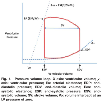
Summary : This figure presents a pressure–volume loop of the left ventricle, illustrating key cardiac parameters such as end-diastolic volume (EDV), end-systolic volume (ESV), stroke volume (SV), end-diastolic pressure (EDP), end-systolic pressure (ESP), arterial elastance (EA), and end-systolic elastance (Ees). The loop visually demonstrates the relationship between ventricular pressure and volume during a cardiac cycle. line plot: # Title & Axes : • Title: "Pressure–volume loop." • X-axis: "Ventricular Volume" (units not specified). – Tick labels: Vo (volume intercept at LV pressure of zero), ESV (end-systolic volume), EDV (end-diastolic volume). • Y-axis: "Ventricular Pressure" (units not specified). – No explicit tick labels shown. # Data & Curve : • Red closed loop traces the pressure–volume relationship during a cardiac cycle. • Horizontal arrow within the loop labeled "SV" (stroke volume) indicates the difference between EDV and ESV. • Vertical segments at EDV and ESV mark transitions between phases. • Dotted lines: – EA (arterial elastance) shown as a dashed line from Vo through ESP/SV. – Ees (end-systolic elastance) shown as a dashed line from Vo through ESP/(ESV-Vo). # Key Parameters & Annotations : • Vo: Volume intercept at LV pressure of zero (leftmost point on x-axis). • ESV: End-systolic volume (right vertical segment). • EDV: End-diastolic volume (far right on x-axis). • SV: Stroke volume (horizontal arrow between ESV and EDV). • EDP: End-diastolic pressure (arrow at bottom right of loop). • ESP: End-systolic pressure (top of loop). • EA: Arterial elastance (dashed line labeled EA (ESP/SV)). • Ees: End-systolic elastance (dashed line labeled Ees = ESP/(ESV-Vo)). # Design Encodings : • Red solid line for the pressure–volume loop. • Blue dashed lines for elastance relationships. • Arrows and labels for key parameters. • No gridlines or axis units specified. # Analysis : • The pressure–volume loop demonstrates the cardiac cycle phases, with the lower right corner representing end-diastole (high volume, low pressure) and the upper left corner representing end-systole (low volume, high pressure). • Stroke volume is visually indicated as the horizontal distance between EDV and ESV. • Elastance lines (EA and Ees) provide graphical representations of arterial and ventricular contractility. • The loop’s shape and annotations allow for assessment of cardiac function and mechanical properties.
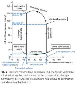
Summary : This figure shows a pressure–volume loop for the left ventricle, illustrating how ventricular volume and pressure change during the cardiac cycle, with key phases and valve events annotated. The isovolumetric relaxation and contraction periods are highlighted, and systolic/diastolic blood pressures are marked. pressure–volume loop diagram: # Title & Axes : • No explicit title on the figure, but the legend describes it as a "Pressure–volume loop demonstrating changes in ventricular volume during filling and ejection with corresponding changes in intracavity pressure." • X-axis: "Left ventricular volume (mL)" with tick marks at 0, 20, 40, 60, 80, 100, 120, 140, 160. • Y-axis: "Left ventricular pressure (mmHg)" with tick marks at 0, 20, 40, 60, 80, 100, 120, 140. • Additional axis labels: "Left ventricular end-diastolic pressure" (blue, left), "End-diastolic volume" (blue, bottom right), "Stroke volume" (black, bottom center). # Phases & Events : • Isovolumetric relaxation: vertical line at low volume, pressure drops, labeled. • Diastolic filling: horizontal line at low pressure, volume increases, labeled. • Isovolumetric contraction: vertical line at high volume, pressure rises, labeled. • Ventricular ejection: curved line, volume decreases as pressure peaks and falls, labeled. • Valve events: – Mitral valve opens (bottom left corner, low pressure/volume). – Mitral valve closes (bottom right corner, high volume/low pressure). – Aortic valve opens (top right corner, high volume/high pressure). – Aortic valve closes (top left corner, low volume/high pressure). # Blood Pressure Markers : • Systolic BP: horizontal dashed blue line at ~120 mmHg. • Diastolic BP: horizontal dashed blue line at ~80 mmHg. # Design Encodings : • Black solid lines for the loop. • Blue dashed lines for blood pressure markers. • Blue text for end-diastolic volume/pressure. • Labeled arrows for direction of phases and valve events. # Analysis : • The loop traces the cardiac cycle, starting at low pressure/volume (end-systolic), filling during diastole, rising sharply during isovolumetric contraction, ejecting blood during ventricular ejection, and dropping pressure during isovolumetric relaxation. • Systolic and diastolic blood pressures are marked, showing the pressure range during ejection. • The width of the loop (horizontal distance) represents stroke volume. • The figure clearly distinguishes the four main phases and the timing of valve openings/closings, providing a comprehensive view of ventricular mechanics during a heartbeat.
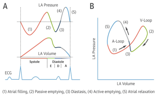
Summary : This figure illustrates the left atrial (LA) pressure-volume relationship during the cardiac cycle, showing both time-course traces and a pressure-volume loop, with key phases of atrial function annotated and correlated with the ECG. line plot and loop diagram: # Panel A: LA Pressure and Volume Traces • Top trace: LA Pressure (y-axis, arbitrary units) over time. • Middle trace: LA Volume (y-axis, arbitrary units) over time. • Bottom trace: ECG waveform for temporal reference. • X-axis: Cardiac cycle phases, with systole and diastole labeled; diastole further subdivided into E, D, and A phases. • Five phases are color-coded and numbered: – (1) Atrial filling (red) – (2) Passive emptying (green) – (3) Diastasis (black) – (4) Active emptying (blue) – (5) Atrial relaxation (gray) • Vertical dashed lines demarcate transitions between phases. # Panel B: LA Pressure-Volume Loop • X-axis: LA Volume (arbitrary units). • Y-axis: LA Pressure (arbitrary units). • The loop is traced in a counterclockwise direction, with arrows indicating the sequence. • The same five phases (1–5) are color-coded as in Panel A. • The loop is divided into two segments: A-Loop (phases 1, 3, 4, 5) and V-Loop (phase 2). # Design Encodings : • Distinct colors for each phase (red, green, black, blue, gray). • Arrows on the loop indicate the direction of the cardiac cycle. • ECG trace provides timing reference for the pressure and volume changes. # Analysis : • The LA pressure and volume traces show cyclical changes corresponding to atrial filling, emptying, and relaxation. • The pressure-volume loop visually summarizes the dynamic relationship between LA pressure and volume, with distinct segments for passive and active phases. • The figure highlights the temporal coordination between atrial events and the ECG, emphasizing the mechanical and electrical coupling in the cardiac cycle.
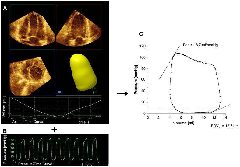
Educational composite image illustrating the generation of ventricular pressure-volume loops (PVL) from diagnostic data. Panel A displays three-dimensional real-time echocardiography (3DE) data, featuring multi-plane apical and short-axis sectional views of the left ventricle alongside a 3D volumetric reconstruction. Below this is a volume-time curve (ml vs. s) tracking ventricular filling and emptying. Panel B presents a pressure-time curve (mmHg vs. s) derived from an invasive mini-pressure wire. Panel C shows the integrated result: a pressure-volume loop mapping the cardiac cycle. Key hemodynamic indices are identified on the PVL, including end-systolic elastance (Ees = 18.7 ml/mmHg), represented by the slope of the end-systolic pressure-volume relationship, and the indexed end-diastolic volume at 10 mmHg (EDV10 = 13.51 ml). This figure demonstrates the methodology for assessing cardiac contractility and compliance by synchronizing non-invasive volumetric imaging with invasive manometry.
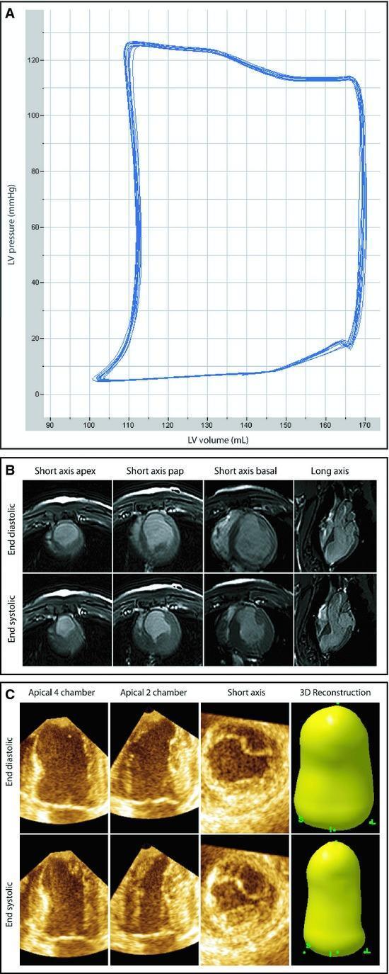
Educational composite figure demonstrating multimodal assessment of left ventricular (LV) function and volume. Panel A shows a Pressure-Volume (PV) loop graph plotting LV pressure (mmHg) against LV volume (mL), characteristic of cardiac cycle analysis. Panel B displays Cardiac Magnetic Resonance Imaging (CMRI) in a 2x4 grid comparing end-diastolic and end-systolic phases across four planes: short-axis apex, papillary muscle level, basal level, and long-axis view. These views highlight ventricular wall thickening and chamber reduction during systole. Panel C illustrates Three-Dimensional Echocardiography (3DE) including apical 4-chamber, apical 2-chamber, and short-axis views alongside a computed 3D reconstruction of the LV volume. The contrast between end-diastolic and end-systolic frames in both CMRI and 3DE allows for the calculation of stroke volume and ejection fraction. The figure serves as a comparative reference for diagnostic imaging modalities used in cardiology to quantify cardiac remodeling and performance after myocardial injury.
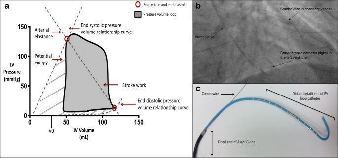
A multi-panel figure illustrating invasive cardiac hemodynamic assessment. Panel (a) is a cardiovascular physiology graph showing a left ventricular (LV) pressure-volume loop. The y-axis represents LV pressure (mmHg) and the x-axis represents LV volume (mL). Key metrics are labeled: the shaded interior represents stroke work (SW); the slopes of the dashed lines define the end-systolic pressure-volume relationship (ESPVR), reflecting contractility, and the end-diastolic pressure-volume relationship (EDPVR), reflecting compliance. Panel (b) is an in-vivo fluoroscopic image in a posteroanterior (PA) view, demonstrating real-time simultaneous data acquisition. It shows a Combowire positioned within a coronary vessel and a conductance catheter (CC) pigtail at the LV apex, with the aortic valve serving as a landmark. Panel (c) provides an ex-vivo photograph of the specialized instrumentation, including the distal end of an Asahi sheathless guide, the Combowire, and the pigtail conductance catheter used for LV pressure-volume analysis. The figure serves to demonstrate the methodology for gold-standard clinical research into cardiac-coronary interactions and hemodynamics.
Frank-Starling law preload afterload contractility cardiac output
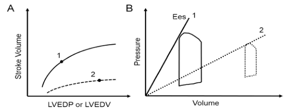
Summary : This figure compares cardiac function under two conditions using two types of plots: (A) the Frank-Starling relationship between stroke volume and left ventricular filling, and (B) pressure-volume loops with end-systolic elastance (Ees) lines. line and schematic plot: # Panel A: Frank-Starling Curve : • Y-axis: Stroke Volume (no units shown). • X-axis: LVEDP or LVEDV (Left Ventricular End-Diastolic Pressure or Volume; no units shown). • Two curves are shown: – Curve 1: Higher, solid line, labeled "1". – Curve 2: Lower, dashed line, labeled "2". • Each curve has a point marked (solid dot) on it. # Panel B: Pressure-Volume Loop and End-Systolic Elastance : • Y-axis: Pressure (no units shown). • X-axis: Volume (no units shown). • Two pressure-volume loops: – Loop 1: Solid line, larger, leftward, labeled "1". – Loop 2: Dashed line, smaller, rightward, labeled "2". • Two Ees (end-systolic elastance) lines: – Ees 1: Steeper, solid line, labeled "1". – Ees 2: Less steep, dashed line, labeled "2". # Design Encodings : • Solid lines for condition 1, dashed lines for condition 2. • Dots mark specific points on the curves in panel A. • Pressure-volume loops are outlined, with loop 2 shown as a dashed outline. # Analysis : • Panel A shows that condition 1 (solid line) has a higher stroke volume for any given LVEDP/LVEDV compared to condition 2 (dashed line), indicating better cardiac function. • Panel B shows that condition 1 has a larger, leftward pressure-volume loop and a steeper Ees line, indicating greater contractility. Condition 2 has a smaller, rightward loop and a less steep Ees line, indicating reduced contractility. • The figure visually contrasts normal/enhanced versus impaired cardiac function using both stroke volume response and pressure-volume relationships.
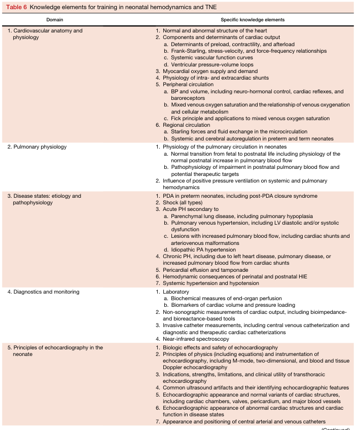
Table 6 Knowledge elements for training in neonatal hemodynamics and TNE <table><thead><tr><th>Domain</th><th>Specific knowledge elements</th></tr></thead><tbody><tr><td>1. Cardiovascular anatomy and physiology</td><td>1. Normal and abnormal structure of the heart<br>2. Components and determinants of cardiac output<br> a. Determinants of preload, contractility, and afterload<br> b. Frank-Starling, stress-velocity, and force-frequency relationships<br> c. Systemic vascular function curves<br> d. Ventricular pressure-volume loops<br>3. Myocardial oxygen supply and demand<br>4. Physiology of intra- and extracardiac shunts<br>5. Peripheral circulation<br> a. BP and volume, including neuro-hormonal control, cardiac reflexes, and baroreceptors<br> b. Mixed venous oxygen saturation and the relationship of venous oxygenation and cellular metabolism<br> c. Fick principle and applications to mixed venous oxygen saturation<br>6. Regional circulation<br> a. Starling forces and fluid exchange in the microcirculation<br> b. Systemic and cerebral autoregulation in preterm and term neonates</td></tr><tr><td>2. Pulmonary physiology</td><td>1. Physiology of the pulmonary circulation in neonates<br> a. Normal transition from fetal to postnatal life including physiology of the normal postnatal increase in pulmonary blood flow<br> b. Pathophysiology of impairment in postnatal pulmonary blood flow and potential therapeutic targets<br>2. Influence of positive pressure ventilation on systemic and pulmonary hemodynamics</td></tr><tr><td>3. Disease states: etiology and pathophysiology</td><td>1. PDA in preterm neonates, including post-PDA closure syndrome<br>2. Shock (all types)<br>3. Acute PH secondary to<br> a. Parenchymal lung disease, including pulmonary hypoplasia<br> b. Pulmonary venous hypertension, including LV diastolic and/or systolic dysfunction<br> c. Lesions with increased pulmonary blood flow, including cardiac shunts and arteriovenous malformations<br> d. Idiopathic PA hypertension<br>4. Chronic PH, including due to left heart disease, pulmonary disease, or increased pulmonary blood flow from cardiac shunts<br>5. Pericardial effusion and tamponade<br>6. Hemodynamic consequences of perinatal and postnatal HIE<br>7. Systemic hypertension and hypotension</td></tr><tr><td>4. Diagnostics and monitoring</td><td>1. Laboratory<br> a. Biochemical measures of end-organ perfusion<br> b. Biomarkers of cardiac volume and pressure loading<br>2. Non-sonographic measurements of cardiac output, including bioimpedance- and bioreactance-based tools<br>3. Invasive catheter measurements, including central venous catheterization and diagnostic and therapeutic cardiac catheterizations<br>4. Near-infrared spectroscopy</td></tr><tr><td>5. Principles of echocardiography in the neonate</td><td>1. Biologic effects and safety of echocardiography<br>2. Principles of physics (including equations) and instrumentation of echocardiography, including M-mode, two-dimensional, and blood and tissue Doppler echocardiography<br>3. Indications, strengths, limitations, and clinical utility of transthoracic echocardiography<br>4. Common ultrasound artifacts and their identifying echocardiographic features<br>5. Echocardiographic appearance and normal variants of cardiac structures, including cardiac chambers, valves, pericardium, and major blood vessels<br>6. Echocardiographic appearance of abnormal cardiac structures and cardiac function in disease states<br>7. Appearance and positioning of central arterial and venous catheters</td></tr></tbody></table>
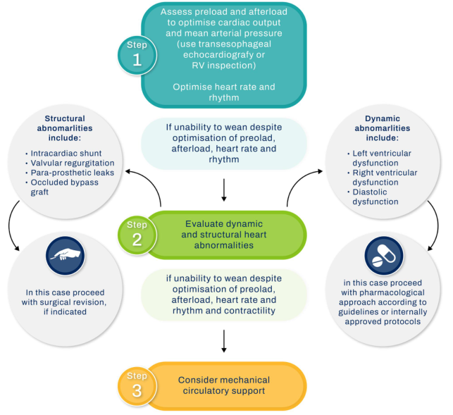
Summary : This flowchart outlines a stepwise approach for managing patients who are difficult to wean from cardiopulmonary bypass, focusing on the assessment and optimization of cardiac function, identification of structural and dynamic heart abnormalities, and escalation to surgical or pharmacological interventions, with consideration of mechanical circulatory support as a final step. flowchart: # Nodes : • Step 1 (rounded rectangle): "Assess preload and afterload to optimise cardiac output and mean arterial pressure (use transesophageal echocardiography or RV inspection). Optimise heart rate and rhythm." • Decision (rectangle): "If inability to wean despite optimisation of preload, afterload, heart rate and rhythm" • Step 2 (rounded rectangle): "Evaluate dynamic and structural heart abnormalities" • Decision (rectangle): "If inability to wean despite optimisation of preload, afterload, heart rate and rhythm and contractility" • Step 3 (rounded rectangle): "Consider mechanical circulatory support" • Structural abnormalities (circle): "Structural abnormalities include: Intracardiac shunt, Valvular regurgitation, Para-prosthetic leaks, Occluded bypass graft" • Surgical revision (circle): "In this case proceed with surgical revision, if indicated" • Dynamic abnormalities (circle): "Dynamic abnormalities include: Left ventricular dysfunction, Right ventricular dysfunction, Diastolic dysfunction" • Pharmacological approach (circle): "In this case proceed with pharmacological approach according to guidelines or internally approved protocols" # Connectors : • Downward arrows connect each step in sequence (Step 1 → Step 2 → Step 3). • From the decision points after Step 1 and Step 2, arrows branch to the left (structural abnormalities) and right (dynamic abnormalities). • From "Structural abnormalities" node, arrow leads to "Surgical revision" node. • From "Dynamic abnormalities" node, arrow leads to "Pharmacological approach" node. # Layout : • The flowchart is vertically oriented with three main steps in the center. • At each decision point, the chart branches horizontally to the left (structural) and right (dynamic) for further evaluation and intervention. • Circular nodes for abnormalities and interventions are placed laterally, with arrows looping back to the main flow as appropriate. # Analysis : • The flowchart provides a logical, stepwise escalation for managing failure to wean from cardiopulmonary bypass. • It emphasizes initial optimization of hemodynamics, followed by targeted evaluation for structural or dynamic cardiac issues. • Interventions are tailored: surgical for structural problems, pharmacological for dynamic dysfunction. • If all else fails, mechanical circulatory support is considered as a last resort.
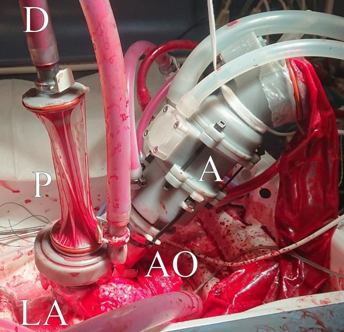
A procedural photograph documenting an ex vivo working heart model setup for hemodynamic research. The central anatomical focus is an isolated heart partially submerged in a perfusate reservoir. On the right, a mechanical afterload device (A), likely based on a Windkessel model, is securely attached to the aorta (AO). This device is a gray, rigid-shelled component containing a compliant internal cuff designed to simulate peripheral resistance and aortic compliance. On the left, a preload component (P) is connected to the left atrium (LA) via a transparent, bulbous vessel, which serves as a compliant sleeve to manage atrial filling. A de-airing mechanism (D) is integrated above the preload to ensure the removal of air bubbles from the circuit. The system is interconnected by a series of transparent and pink-hued tubes carrying oxygenated perfusate. This experimental apparatus is designed to replicate physiological systolic and diastolic pressure limits and aortic pressure waveforms in an isolated heart environment, typically used for evaluating cardiac power, valve function, or pharmacological responses.
cardiac action potential phases myocardial excitation contraction coupling calcium
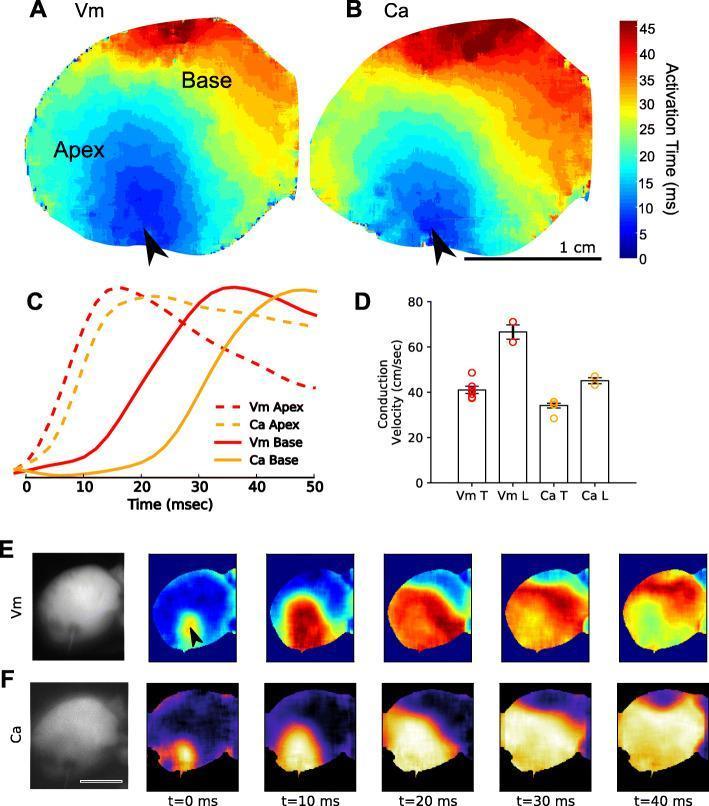
This composite educational graphic illustrates multiparametric optical mapping of cardiac excitation-contraction coupling in an isolated heart model. Panels A and B present isochronal activation maps for transmembrane voltage (Vm) and intracellular calcium (Ca), respectively, showing impulse propagation from the apex (blue) to the base (red) over a 45 ms scale. Panel C displays representative signal upstroke traces, highlighting the physiological lag between electrical depolarization (Vm) and calcium release (Ca) at both the apex and base. Panel D provides a bar chart comparing transverse (T) and longitudinal (L) conduction velocities for Vm and Ca, indicating significantly faster longitudinal Vm propagation compared to Ca. Panels E and F show sequential time-lapse frames (t=0 to 40 ms) of wavefront propagation following electrical pacing at the apex (indicated by arrows). These frames demonstrate the development of spatial heterogeneity and wavebreak in the calcium channel at t=40 ms, serving as a model for studying electrophysiological discontinuities and potential arrhythmogenic precursors.
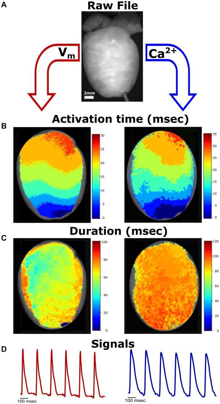
This composite educational graphic illustrates the workflow for cardiac optical mapping, specifically focusing on the simultaneous analysis of transmembrane voltage (Vm) and intracellular calcium (Ca2+) in a mammalian heart model. Panel A shows the raw grayscale image of a Langendorff-perfused heart. Panel B presents activation time maps in milliseconds (msec) for both Vm and Ca2+. These pseudocolor maps demonstrate the propagation of electrical and calcium signals from the apex (blue, indicating earlier activation) toward the base (red, indicating later activation), reflecting the coordinated cardiac conduction sequence. Panel C displays duration maps for the action potential and calcium transients. The Vm duration map (left) utilizes a scale up to 100 msec, while the Ca2+ duration map (right) extends to 120 msec, highlighting the characteristically longer duration of calcium transients. Panel D provides representative temporal signal traces, showing the morphology of repetitive action potentials and calcium transients. This figure serves as a diagnostic tool for evaluating excitation-contraction coupling and regional heterogeneity in cardiac electrophysiology.
![This composite educational image illustrates an experimental cardiac electrophysiology preparation. Panel A shows a clinical photograph of a dissected left atrial (LA) endocardial surface. Key anatomical regions are labeled, including the left atrial appendage (LAA) on the left, the pulmonary veins (PV) on the right, and the free wall (FW) at the inferior margin. A dotted white line outlines the mapped atrial tissue, and an arrow indicates the site of left circumflex (LCx) coronary artery perfusion. A 1 cm scale bar is provided for reference. Panel B displays simultaneous representative physiological signals recorded during atrial pacing at a cycle length of 1000 ms. The waveforms include a pseudo-ECG (black), optical action potentials (Vm, blue) showing rapid upstroke and repolarization phases, and intracellular calcium transients ([Ca2+]i, red) demonstrating calcium release and sequestration. The alignment of the signals illustrates the excitation-contraction coupling sequence, where the electrical action potential (Vm) precedes the rise in the calcium transient. A 1-second scale bar confirms the temporal pacing interval.](https://cdn.orris.care/cdss_images/pmc_clinical_VQA_3e2599ba302fee4a831f8f4d382a4769320d1c53308a487c0be6a60df7c710bf.jpg)
This composite educational image illustrates an experimental cardiac electrophysiology preparation. Panel A shows a clinical photograph of a dissected left atrial (LA) endocardial surface. Key anatomical regions are labeled, including the left atrial appendage (LAA) on the left, the pulmonary veins (PV) on the right, and the free wall (FW) at the inferior margin. A dotted white line outlines the mapped atrial tissue, and an arrow indicates the site of left circumflex (LCx) coronary artery perfusion. A 1 cm scale bar is provided for reference. Panel B displays simultaneous representative physiological signals recorded during atrial pacing at a cycle length of 1000 ms. The waveforms include a pseudo-ECG (black), optical action potentials (Vm, blue) showing rapid upstroke and repolarization phases, and intracellular calcium transients ([Ca2+]i, red) demonstrating calcium release and sequestration. The alignment of the signals illustrates the excitation-contraction coupling sequence, where the electrical action potential (Vm) precedes the rise in the calcium transient. A 1-second scale bar confirms the temporal pacing interval.
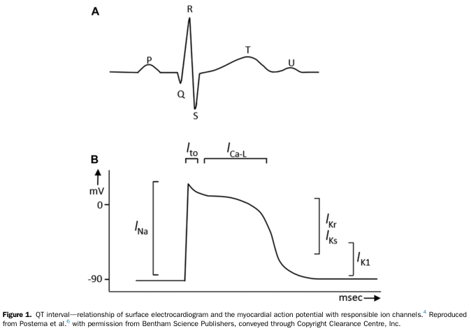
Summary : This figure illustrates the relationship between the surface electrocardiogram (ECG) waveform and the myocardial action potential, highlighting the corresponding ion channels responsible for different phases of cardiac electrical activity. line diagram: # Panel A: Surface Electrocardiogram (ECG) Waveform : • Shows a typical ECG trace with labeled points: P, Q, R, S, T, and U. • The waveform represents the electrical activity of the heart during a cardiac cycle. • P wave: atrial depolarization. • QRS complex: ventricular depolarization. • T wave: ventricular repolarization. • U wave: sometimes seen, origin not fully understood. # Panel B: Myocardial Action Potential : • Plots membrane potential (mV) on the y-axis (ranging from -90 mV to above 0 mV) against time (msec) on the x-axis. • Shows the phases of the cardiac action potential: – Rapid upstroke (depolarization) due to I_Na (sodium current). – Early repolarization (I_to, transient outward potassium current). – Plateau phase (I_Ca-L, L-type calcium current). – Repolarization phase (I_Kr and I_Ks, rapid and slow delayed rectifier potassium currents). – Resting potential maintained by I_K1 (inward rectifier potassium current). # Ion Channels & Phases : • I_Na: Responsible for the initial rapid depolarization. • I_to: Contributes to early repolarization. • I_Ca-L: Maintains the plateau phase. • I_Kr and I_Ks: Mediate repolarization. • I_K1: Maintains the resting membrane potential. # Design Encodings : • Simple black line traces for both ECG and action potential. • Ion channel names are annotated above the relevant phases of the action potential. # Analysis : • The figure visually links the phases of the ECG waveform to the underlying myocardial action potential and the specific ion channels involved. • The QRS complex corresponds to the rapid depolarization (I_Na), while the T wave aligns with repolarization (I_Kr, I_Ks). • The plateau phase (I_Ca-L) is crucial for the duration of the QT interval, which is clinically significant for arrhythmia risk. • The diagram provides a clear educational overview of how surface ECG features relate to cellular electrophysiology.
mkdir -p /tmp/workspace/cardiac-physiology-ppt
python /tmp/skills/shared/scripts/fetch_images.py \ "https://cdn.orris.care/cdss_images/GLGCA_4716091_1766472504697_d6487393-2ad4-46b0-89dd-781086017023_419c4963-ac36-4b02-b687-a8b38c0b8a8e.png" \ "https://cdn.orris.care/cdss_images/GLGCA_11173_1762898730916_a06e7b2c-afa5-4859-87c0-0a2dc26524e8.png" \ "https://cdn.orris.care/cdss_images/GLGCA_11173_1762898798398_6b9c785a-c63f-46c2-bb11-d9bae18f8286.png" \ "https://cdn.orris.care/cdss_images/GLGCA_4566687_1766513411587_8a5894b1-50f7-44cf-a343-23ce617e9716_17474780-6526-46a8-abb3-4dba8e158f96.png" \ 2>/dev/null | python3 -c "import sys,json; data=json.load(sys.stdin); [print(i, d['base64'][:30] if d['base64'] else 'FAILED') for i,d in enumerate(data)]"
~/cardiac-physiology-ppt/build_ppt.py
import json, subprocess, base64
from io import BytesIO
from pptx import Presentation
from pptx.util import Inches, Pt, Emu
from pptx.dml.color import RGBColor
from pptx.enum.text import PP_ALIGN, MSO_ANCHOR

# ─── Color palette (deep navy / teal / white) ─────────────────────────────────
NAVY    = RGBColor(0x0A, 0x1E, 0x3C)   # slide background
TEAL    = RGBColor(0x00, 0x8B, 0x8B)   # accent / section headers
GOLD    = RGBColor(0xF0, 0xB4, 0x29)   # highlight
WHITE   = RGBColor(0xFF, 0xFF, 0xFF)
LIGHT   = RGBColor(0xE8, 0xF4, 0xF8)   # subtle box background
DARK_T  = RGBColor(0x00, 0x5F, 0x5F)   # darker teal for sub-headers

W = Inches(13.333)
H = Inches(7.5)

def new_prs():
    prs = Presentation()
    prs.slide_width  = W
    prs.slide_height = H
    return prs

def blank_slide(prs, bg=NAVY):
    sl = prs.slides.add_slide(prs.slide_layouts[6])
    fill = sl.background.fill
    fill.solid()
    fill.fore_color.rgb = bg
    return sl

def add_rect(slide, x, y, w, h, color, alpha=None):
    shape = slide.shapes.add_shape(1, x, y, w, h)  # MSO_SHAPE_TYPE.RECTANGLE
    shape.fill.solid()
    shape.fill.fore_color.rgb = color
    shape.line.fill.background()
    return shape

def add_text(slide, text, x, y, w, h, size=18, bold=False, color=WHITE,
             align=PP_ALIGN.LEFT, wrap=True, italic=False):
    tb = slide.shapes.add_textbox(x, y, w, h)
    tf = tb.text_frame
    tf.word_wrap = wrap
    tf.margin_left = Pt(4)
    tf.margin_right = Pt(4)
    tf.margin_top = Pt(2)
    tf.margin_bottom = Pt(2)
    p = tf.paragraphs[0]
    p.alignment = align
    r = p.add_run()
    r.text = text
    r.font.name  = "Calibri"
    r.font.size  = Pt(size)
    r.font.bold  = bold
    r.font.color.rgb = color
    r.font.italic = italic
    return tf

def add_bullet_text(slide, bullets, x, y, w, h, size=16, color=WHITE,
                    title=None, title_size=20, title_color=TEAL):
    tb = slide.shapes.add_textbox(x, y, w, h)
    tf = tb.text_frame
    tf.word_wrap = True
    tf.margin_left = Pt(6)
    tf.margin_right = Pt(4)
    tf.margin_top = Pt(4)
    tf.margin_bottom = Pt(4)

    first = True
    if title:
        p = tf.paragraphs[0]
        p.alignment = PP_ALIGN.LEFT
        r = p.add_run()
        r.text = title
        r.font.name  = "Calibri"
        r.font.size  = Pt(title_size)
        r.font.bold  = True
        r.font.color.rgb = title_color
        first = False

    for bullet in bullets:
        if first:
            p = tf.paragraphs[0]
            first = False
        else:
            p = tf.add_paragraph()
        p.alignment = PP_ALIGN.LEFT
        p.space_before = Pt(4)
        r = p.add_run()
        r.text = f"  \u2022  {bullet}"
        r.font.name  = "Calibri"
        r.font.size  = Pt(size)
        r.font.color.rgb = color
    return tf

def add_image_from_url(slide, url, x, y, w, h):
    result = json.loads(subprocess.check_output(
        ["python", "/tmp/skills/shared/scripts/fetch_images.py", url]
    ))
    img_data = result[0]
    if img_data["base64"]:
        b64 = img_data["base64"]
        if "," in b64:
            b64 = b64.split(",", 1)[1]
        raw = base64.b64decode(b64)
        slide.shapes.add_picture(BytesIO(raw), x, y, width=w, height=h)

def add_divider(slide, y, color=TEAL, thickness=Pt(2)):
    line = slide.shapes.add_connector(1, Inches(0.4), y, Inches(12.93), y)
    line.line.color.rgb = color
    line.line.width = thickness

# ─── Image URLs ───────────────────────────────────────────────────────────────
IMG_PV_LOOP_ANNOTATED = "https://cdn.orris.care/cdss_images/GLGCA_4716091_1766472504697_d6487393-2ad4-46b0-89dd-781086017023_419c4963-ac36-4b02-b687-a8b38c0b8a8e.png"
IMG_PV_LOOP_SIMPLE    = "https://cdn.orris.care/cdss_images/GLGCA_11173_1762898730916_a06e7b2c-afa5-4859-87c0-0a2dc26524e8.png"
IMG_FRANK_STARLING    = "https://cdn.orris.care/cdss_images/GLGCA_11173_1762898798398_6b9c785a-c63f-46c2-bb11-d9bae18f8286.png"
IMG_AP_ION_CHANNELS   = "https://cdn.orris.care/cdss_images/GLGCA_4566687_1766513411587_8a5894b1-50f7-44cf-a343-23ce617e9716_17474780-6526-46a8-abb3-4dba8e158f96.png"

# ═══════════════════════════════════════════════════════════════════════════════
prs = new_prs()

# ─── SLIDE 1: Title ───────────────────────────────────────────────────────────
s1 = blank_slide(prs, NAVY)
add_rect(s1, 0, 0, W, Inches(0.18), TEAL)
add_rect(s1, 0, Inches(7.32), W, Inches(0.18), TEAL)

# Gold accent bar
add_rect(s1, Inches(0), Inches(2.8), Inches(0.12), Inches(2.0), GOLD)

# Main title
add_text(s1, "CARDIAC PHYSIOLOGY",
         Inches(0.4), Inches(2.8), Inches(12.5), Inches(1.2),
         size=54, bold=True, color=WHITE, align=PP_ALIGN.LEFT)

add_text(s1, "Reference: Miller's Anesthesia, 10th Edition",
         Inches(0.4), Inches(4.0), Inches(10), Inches(0.55),
         size=22, color=TEAL, bold=False, align=PP_ALIGN.LEFT)

add_text(s1, "Chapter 13  |  Lena S. Sun & Nicholas A. Davis",
         Inches(0.4), Inches(4.55), Inches(10), Inches(0.45),
         size=18, color=LIGHT, align=PP_ALIGN.LEFT, italic=True)

add_text(s1, "From Harvey's circulation (1628) to modern cellular cardiology",
         Inches(0.4), Inches(5.3), Inches(10), Inches(0.45),
         size=15, color=GOLD, italic=True, align=PP_ALIGN.LEFT)

# ─── SLIDE 2: Overview / Key Points ─────────────────────────────────────────
s2 = blank_slide(prs, NAVY)
add_rect(s2, 0, 0, W, Inches(1.1), DARK_T)
add_text(s2, "KEY CONCEPTS", Inches(0.4), Inches(0.15), Inches(12), Inches(0.8),
         size=32, bold=True, color=WHITE)
add_divider(s2, Inches(1.1))

kp = [
    "Cardiac cycle = sequence of electrical & mechanical events in a single heartbeat",
    "Cardiac output determined by: heart rate, contractility, preload & afterload",
    "Cardiomyocytes contain myofibrils — the contractile elements; sarcomere is the basic working unit",
    "Gap junctions mediate electrical coupling between cardiomyocytes",
    "Action potentials have four phases in the heart",
    "Key mediator of excitation-contraction coupling: Calcium (Ca²+)",
    "Ca²+-induced sparks regulate automaticity and contractility",
    "Cardiac reflexes = fast loops between heart and CNS maintaining homeostasis",
]
add_bullet_text(s2, kp, Inches(0.4), Inches(1.2), Inches(12.5), Inches(6.0),
                size=17, color=WHITE)

# ─── SLIDE 3: Cardiac Cycle ───────────────────────────────────────────────────
s3 = blank_slide(prs, NAVY)
add_rect(s3, 0, 0, W, Inches(1.0), DARK_T)
add_text(s3, "THE CARDIAC CYCLE", Inches(0.3), Inches(0.1), Inches(12), Inches(0.8),
         size=30, bold=True, color=WHITE)
add_divider(s3, Inches(1.0))

# Left column
left_bullets = [
    "Sequence of electrical & mechanical events during one heartbeat",
    "P wave: atrial depolarization",
    "QRS complex: ventricular depolarization",
    "T wave: ventricular repolarization",
    "",
    "PHASES OF THE CARDIAC CYCLE:",
    "1.  Isovolumetric Contraction",
    "     - Mitral & tricuspid close; aortic/pulmonic still closed",
    "     - LV pressure rises rapidly",
    "2.  Rapid Ejection",
    "     - Aortic/pulmonic valves open; SV ejected",
    "3.  Isovolumetric Relaxation",
    "     - Aortic valve closes (dicrotic notch); LV relaxes",
    "4.  Rapid Ventricular Filling",
    "     - Mitral opens; passive filling (70% of SV)",
    "5.  Atrial Contraction (Systole)",
    "     - Active filling; contributes 20-30% of EDV",
]
add_bullet_text(s3, left_bullets, Inches(0.3), Inches(1.1), Inches(6.8), Inches(6.2),
                size=14.5, color=WHITE)

# Right: PV loop image
try:
    add_image_from_url(s3, IMG_PV_LOOP_ANNOTATED, Inches(7.2), Inches(1.1), Inches(5.8), Inches(5.9))
except:
    add_text(s3, "[P-V Loop Diagram]", Inches(7.2), Inches(3.0), Inches(5.8), Inches(1.0),
             size=16, color=TEAL, align=PP_ALIGN.CENTER)

add_text(s3, "Source: Miller's Anesthesia 10e, Chapter 13",
         Inches(0.3), Inches(7.1), Inches(12), Inches(0.35),
         size=10, color=TEAL, italic=True)

# ─── SLIDE 4: Ventricular Function & PV Loop ─────────────────────────────────
s4 = blank_slide(prs, NAVY)
add_rect(s4, 0, 0, W, Inches(1.0), DARK_T)
add_text(s4, "PRESSURE-VOLUME LOOP & VENTRICULAR FUNCTION",
         Inches(0.3), Inches(0.1), Inches(12.7), Inches(0.8),
         size=26, bold=True, color=WHITE)
add_divider(s4, Inches(1.0))

# Left: PV loop simple
try:
    add_image_from_url(s4, IMG_PV_LOOP_SIMPLE, Inches(0.3), Inches(1.1), Inches(5.5), Inches(5.5))
except:
    pass

# Right: annotations
pv_points = [
    "EDV: End-diastolic volume (preload)",
    "ESV: End-systolic volume",
    "SV = EDV - ESV  (normal ~70 mL)",
    "EF = SV / EDV  (normal >55%)",
    "",
    "ESPVR slope (Ees): index of contractility",
    "EDPVR: diastolic compliance curve",
    "Arterial Elastance (Ea): afterload",
    "Stroke Work = area within PV loop",
    "",
    "Preload increase => rightward loop shift",
    "Afterload increase => smaller loop, higher ESP",
    "Positive inotropy => steeper Ees, larger SV",
]
add_bullet_text(s4, pv_points, Inches(6.0), Inches(1.1), Inches(7.0), Inches(6.0),
                size=15.5, color=WHITE, title="PV Loop Parameters",
                title_size=19, title_color=GOLD)

add_text(s4, "Source: Miller's Anesthesia 10e, Chapter 13",
         Inches(0.3), Inches(7.1), Inches(12), Inches(0.35),
         size=10, color=TEAL, italic=True)

# ─── SLIDE 5: Determinants of Cardiac Output ─────────────────────────────────
s5 = blank_slide(prs, NAVY)
add_rect(s5, 0, 0, W, Inches(1.0), DARK_T)
add_text(s5, "DETERMINANTS OF CARDIAC OUTPUT",
         Inches(0.3), Inches(0.1), Inches(12.7), Inches(0.8),
         size=28, bold=True, color=WHITE)
add_divider(s5, Inches(1.0))

# CO equation box
add_rect(s5, Inches(0.3), Inches(1.1), Inches(12.7), Inches(0.65), TEAL)
add_text(s5, "CO = HR × SV          Normal: 4-8 L/min          CI = CO / BSA  (Normal: 2.4-4.0 L/min/m²)",
         Inches(0.3), Inches(1.1), Inches(12.7), Inches(0.65),
         size=18, bold=True, color=WHITE, align=PP_ALIGN.CENTER)

# 4 boxes: HR, Preload, Afterload, Contractility
box_data = [
    ("HEART RATE", TEAL, [
        "Normal: 60-100 bpm",
        "Extrinsic control: ANS",
        "SA node pacemaker: 60-100/min",
        "AV node: 40-60/min backup",
        "Tachycardia: reduces diastolic filling time",
        "Bradycardia: increases SV but lowers CO",
    ]),
    ("PRELOAD", DARK_T, [
        "= LVEDV or LVEDP",
        "Frank-Starling Law: increased preload",
        "  => increased stretch => more force",
        "Determinants: venous return, blood volume,",
        "  atrial contraction, myocardial compliance",
        "Monitored by PCWP / CVP",
    ]),
    ("AFTERLOAD", DARK_T, [
        "= Resistance to ventricular ejection",
        "Left ventricle: SVR (systemic vascular resistance)",
        "Right ventricle: PVR (pulmonary vascular resistance)",
        "Increased afterload => reduced SV",
        "SVR = (MAP - CVP) / CO × 80",
        "Normal SVR: 800-1200 dyn·sec·cm⁻⁵",
    ]),
    ("CONTRACTILITY", TEAL, [
        "= Intrinsic myocardial force",
        "(independent of preload/afterload)",
        "Increased by: catecholamines, Ca²+",
        "  digoxin, sympathetic stimulation",
        "Decreased by: heart failure, acidosis,",
        "  beta-blockers, volatile anesthetics",
        "Index: Ees (ESPVR slope), dP/dt max",
    ]),
]

bx_w = Inches(3.1)
bx_h = Inches(4.5)
bx_y = Inches(1.85)
for i, (title, color, bullets) in enumerate(box_data):
    bx_x = Inches(0.3 + i * 3.25)
    add_rect(s5, bx_x, bx_y, bx_w, bx_h, color)
    add_text(s5, title, bx_x, bx_y + Inches(0.05), bx_w, Inches(0.55),
             size=16, bold=True, color=WHITE, align=PP_ALIGN.CENTER)
    add_rect(s5, bx_x, bx_y + Inches(0.58), bx_w, Inches(0.03), GOLD)
    add_bullet_text(s5, bullets,
                    bx_x + Inches(0.05), bx_y + Inches(0.65),
                    bx_w - Inches(0.1), bx_h - Inches(0.7),
                    size=13, color=WHITE)

add_text(s5, "Source: Miller's Anesthesia 10e, Chapter 13",
         Inches(0.3), Inches(7.1), Inches(12), Inches(0.35),
         size=10, color=TEAL, italic=True)

# ─── SLIDE 6: Frank-Starling Law ─────────────────────────────────────────────
s6 = blank_slide(prs, NAVY)
add_rect(s6, 0, 0, W, Inches(1.0), DARK_T)
add_text(s6, "FRANK-STARLING LAW OF THE HEART",
         Inches(0.3), Inches(0.1), Inches(12.7), Inches(0.8),
         size=28, bold=True, color=WHITE)
add_divider(s6, Inches(1.0))

# Left column: text
fs_bullets = [
    "The heart automatically adjusts its output to match venous return",
    "Greater diastolic filling (preload) => increased sarcomere stretch",
    "=> Enhanced actin-myosin cross-bridge formation",
    "=> Greater contractile force and stroke volume",
    "",
    "Optimal sarcomere length: 2.0-2.2 µm",
    "  - Best overlap between actin and myosin filaments",
    "  - Maximum calcium sensitivity of troponin C",
    "",
    "CLINICAL SIGNIFICANCE:",
    "  - Basis for fluid resuscitation in shock",
    "  - Right and left ventricle outputs are balanced",
    "  - Heart failure: depressed Starling curve",
    "  - Positive inotropy: upward shift of curve",
    "",
    "Cardiac Work (Starling): O2 consumption correlates",
    "  with ventricular pressure x volume (not flow alone)",
]
add_bullet_text(s6, fs_bullets, Inches(0.3), Inches(1.1), Inches(6.5), Inches(6.2),
                size=14.5, color=WHITE)

# Right: Frank-Starling image
try:
    add_image_from_url(s6, IMG_FRANK_STARLING, Inches(6.8), Inches(1.1), Inches(6.2), Inches(5.8))
except:
    add_text(s6, "[Frank-Starling Curve]", Inches(6.8), Inches(3.5), Inches(6.2), Inches(1.0),
             size=16, color=TEAL, align=PP_ALIGN.CENTER)

add_text(s6, "Source: Miller's Anesthesia 10e, Chapter 13",
         Inches(0.3), Inches(7.1), Inches(12), Inches(0.35),
         size=10, color=TEAL, italic=True)

# ─── SLIDE 7: Cardiac Work & Oxygen Consumption ──────────────────────────────
s7 = blank_slide(prs, NAVY)
add_rect(s7, 0, 0, W, Inches(1.0), DARK_T)
add_text(s7, "CARDIAC WORK & MYOCARDIAL O₂ CONSUMPTION",
         Inches(0.3), Inches(0.1), Inches(12.7), Inches(0.8),
         size=26, bold=True, color=WHITE)
add_divider(s7, Inches(1.0))

# Left column
work_bullets = [
    "STROKE WORK (SW):",
    "  SW = SV × MAP  (approx.)",
    "  = Area within the PV loop",
    "  Normal LVSW: 60-80 g·m/beat",
    "",
    "CARDIAC WORK (CW):",
    "  CW = CO × MAP × 0.0144",
    "  Normal: ~3-5 kg·m/min",
    "",
    "MYOCARDIAL O₂ DEMAND (MVO₂):",
    "  Determinants: Heart rate (most important!)",
    "  Wall stress (Laplace: T = P×r / 2h)",
    "  Contractility",
    "  Basal metabolism (20% of total MVO₂)",
    "",
    "OXYGEN SUPPLY:",
    "  Coronary blood flow occurs mainly in diastole",
    "  Coronary perfusion pressure = AoP - LVEDP",
    "  O₂ extraction already near maximum at rest",
    "  Increased demand met by increased flow only",
]
add_bullet_text(s7, work_bullets, Inches(0.3), Inches(1.1), Inches(6.3), Inches(6.2),
                size=14, color=WHITE)

# Right column - key formulas box
add_rect(s7, Inches(6.6), Inches(1.15), Inches(6.5), Inches(6.2), RGBColor(0x0D, 0x2E, 0x56))
fmls = [
    "FICK PRINCIPLE:",
    "CO = VO₂ / (CaO₂ - CvO₂)",
    "  VO₂ = O₂ consumption (mL/min)",
    "  CaO₂ = arterial O₂ content",
    "  CvO₂ = venous O₂ content",
    "",
    "O₂ CONTENT:",
    "CaO₂ = (Hb × 1.34 × SaO₂) + (0.003 × PaO₂)",
    "Normal: ~20 mL/dL",
    "",
    "OXYGEN DELIVERY (DO₂):",
    "DO₂ = CO × CaO₂ × 10",
    "Normal: ~1000 mL/min",
    "",
    "OXYGEN EXTRACTION RATIO:",
    "O₂ER = VO₂ / DO₂  (Normal: ~25%)",
    "",
    "DOUBLE PRODUCT (Rate-Pressure Product):",
    "RPP = HR × SBP",
    "  Correlates with MVO₂",
    "  Angina threshold: RPP ~20,000",
]
add_bullet_text(s7, fmls, Inches(6.8), Inches(1.3), Inches(6.1), Inches(5.9),
                size=13.5, color=WHITE)

add_text(s7, "Source: Miller's Anesthesia 10e, Chapter 13",
         Inches(0.3), Inches(7.1), Inches(12), Inches(0.35),
         size=10, color=TEAL, italic=True)

# ─── SLIDE 8: Cellular Cardiac Physiology ─────────────────────────────────────
s8 = blank_slide(prs, NAVY)
add_rect(s8, 0, 0, W, Inches(1.0), DARK_T)
add_text(s8, "CELLULAR CARDIAC PHYSIOLOGY",
         Inches(0.3), Inches(0.1), Inches(12.7), Inches(0.8),
         size=30, bold=True, color=WHITE)
add_divider(s8, Inches(1.0))

cell_l = [
    "CARDIOMYOCYTE STRUCTURE:",
    "  - 50% of volume = myofibrils (contractile elements)",
    "  - Remainder: mitochondria, nucleus, SR, cytosol",
    "  - Length ~100 µm; diameter ~20 µm",
    "  - Branching structure with intercalated discs",
    "",
    "SARCOMERE (basic contractile unit):",
    "  - Z discs to Z discs; length 2.0-2.2 µm at rest",
    "  - Thick filaments: myosin (heavy & light chains)",
    "  - Thin filaments: actin + troponin + tropomyosin",
    "  - Titin: elastic spring linking myosin to Z disc",
    "",
    "INTERCALATED DISCS:",
    "  - Gap junctions: electrical coupling (connexin-43)",
    "  - Desmosomes: mechanical linkage",
    "  - Fasciae adherens: anchor contractile apparatus",
    "",
    "SARCOPLASMIC RETICULUM (SR):",
    "  - Internal Ca²+ store",
    "  - Terminal cisternae adjacent to T-tubules",
    "  - RyR2 (ryanodine receptor): Ca²+ release channel",
    "  - SERCA2a: Ca²+ reuptake ATPase",
]
add_bullet_text(s8, cell_l, Inches(0.3), Inches(1.1), Inches(7.0), Inches(6.2),
                size=13.5, color=WHITE)

cell_r = [
    "MYOSIN ISOFORMS:",
    "  - α-MHC (V1): fast; β-MHC (V3): slow",
    "  - Humans: predominantly β-MHC in adult ventricle",
    "  - Atria: α-MHC predominates",
    "",
    "REGULATORY PROTEINS:",
    "  - Troponin C: Ca²+ binding site",
    "  - Troponin I: inhibitory subunit",
    "  - Troponin T: attaches to tropomyosin",
    "  - Tropomyosin: blocks actin-myosin site at rest",
    "",
    "CROSS-BRIDGE CYCLE:",
    "  1. Ca²+ binds TnC => troponin conformational change",
    "  2. Tropomyosin moves => actin site exposed",
    "  3. Myosin head binds actin (power stroke)",
    "  4. ATP hydrolysis => detachment",
    "  5. Cycle repeats while Ca²+ elevated",
    "",
    "LENGTH-DEPENDENT ACTIVATION:",
    "  - Sarcomere stretch => higher Ca²+ sensitivity",
    "  - Titin stiffness modulates cross-bridge kinetics",
    "  - Basis of Frank-Starling mechanism at cellular level",
]
add_bullet_text(s8, cell_r, Inches(7.1), Inches(1.1), Inches(6.0), Inches(6.2),
                size=13.5, color=WHITE)

add_text(s8, "Source: Miller's Anesthesia 10e, Chapter 13",
         Inches(0.3), Inches(7.1), Inches(12), Inches(0.35),
         size=10, color=TEAL, italic=True)

# ─── SLIDE 9: Action Potentials ───────────────────────────────────────────────
s9 = blank_slide(prs, NAVY)
add_rect(s9, 0, 0, W, Inches(1.0), DARK_T)
add_text(s9, "CARDIAC ACTION POTENTIALS",
         Inches(0.3), Inches(0.1), Inches(12.7), Inches(0.8),
         size=30, bold=True, color=WHITE)
add_divider(s9, Inches(1.0))

# Left: AP image
try:
    add_image_from_url(s9, IMG_AP_ION_CHANNELS, Inches(0.3), Inches(1.1), Inches(6.5), Inches(5.5))
except:
    pass

# Right: AP table / bullets
ap_bullets = [
    "VENTRICULAR AP (5 phases):",
    "",
    "Phase 0: RAPID DEPOLARIZATION",
    "  - Fast Na+ influx (INa); upstroke to +30 mV",
    "  - Rapid, large; gives conduction velocity",
    "",
    "Phase 1: EARLY REPOLARIZATION",
    "  - Ito (transient outward K+ current)",
    "  - Brief notch before plateau",
    "",
    "Phase 2: PLATEAU",
    "  - ICa-L (L-type Ca²+ influx) balanced by IKr",
    "  - Unique to cardiac muscle; enables EC coupling",
    "  - Duration: ~200-300 ms (prevents tetany!)",
    "",
    "Phase 3: RAPID REPOLARIZATION",
    "  - IKr, IKs (delayed rectifier K+ outflow)",
    "  - Return to resting potential",
    "",
    "Phase 4: RESTING POTENTIAL / PACEMAKER",
    "  - IK1 maintains -90 mV in working myocytes",
    "  - Funny current (If / HCN): pacemaker depol.",
    "  - SA node: phase 4 spontaneous depolarization",
    "",
    "PACEMAKER HIERARCHY:",
    "  SA node (60-100/min) > AV node (40-60/min)",
    "  > His-Purkinje (20-40/min)",
]
add_bullet_text(s9, ap_bullets, Inches(7.0), Inches(1.1), Inches(6.1), Inches(6.1),
                size=13, color=WHITE)

add_text(s9, "Source: Miller's Anesthesia 10e, Chapter 13",
         Inches(0.3), Inches(7.1), Inches(12), Inches(0.35),
         size=10, color=TEAL, italic=True)

# ─── SLIDE 10: Excitation-Contraction Coupling ────────────────────────────────
s10 = blank_slide(prs, NAVY)
add_rect(s10, 0, 0, W, Inches(1.0), DARK_T)
add_text(s10, "EXCITATION-CONTRACTION COUPLING",
         Inches(0.3), Inches(0.1), Inches(12.7), Inches(0.8),
         size=28, bold=True, color=WHITE)
add_divider(s10, Inches(1.0))

ecc_l = [
    "CALCIUM - THE KEY SECOND MESSENGER:",
    "  Resting [Ca²+]i: ~100 nM",
    "  Peak systolic [Ca²+]i: ~1 µM (10x increase)",
    "",
    "EC COUPLING STEPS:",
    "1. AP travels along sarcolemma & T-tubules",
    "2. L-type Ca²+ channels (DHPR) open",
    "   => Ca²+ influx (trigger calcium, ~10% of total)",
    "3. RyR2 on SR opens (CICR)",
    "   => Large Ca²+ release from SR (~90%)",
    "4. Ca²+ binds troponin C",
    "   => Cross-bridge cycling begins",
    "5. Relaxation:",
    "   - SERCA2a pumps Ca²+ back into SR",
    "   - NCX (3Na+/1Ca²+) extrudes Ca²+ out of cell",
    "   - Phospholamban regulates SERCA2a activity",
    "",
    "CA²+ SPARKS:",
    "  - Localized SR Ca²+ release events",
    "  - Regulate automaticity & contractility",
    "  - Abnormal sparks => arrhythmias",
]
add_bullet_text(s10, ecc_l, Inches(0.3), Inches(1.1), Inches(6.5), Inches(6.2),
                size=14, color=WHITE)

ecc_r = [
    "PHARMACOLOGICAL TARGETS:",
    "",
    "Ca²+ channel blockers (CCBs):",
    "  Verapamil / Diltiazem: -ve inotropy, chronotropy",
    "  Dihydropyridines (nifedipine): mainly vasodilator",
    "",
    "Beta-blockers:",
    "  Reduce cAMP => less PKA activity",
    "  => Reduced ICa-L, reduced RyR2 phosphorylation",
    "  => Negative inotropy & chronotropy",
    "",
    "Catecholamines (adrenaline/noradrenaline):",
    "  Beta-1 activation => increased cAMP/PKA",
    "  => More ICa-L, more SR Ca²+ release",
    "  => Positive inotrope & chronotrope",
    "",
    "Digoxin:",
    "  Inhibits Na+/K+ ATPase",
    "  => [Na+]i rises => NCX reversed",
    "  => More intracellular Ca²+ => +ve inotropy",
    "",
    "Volatile Anesthetics (e.g. Sevoflurane):",
    "  Reduce ICa-L and Ca²+ sensitivity of myofilaments",
    "  => Dose-dependent negative inotropy",
    "  Isoflurane/Sevoflurane: also cause vasodilation",
]
add_bullet_text(s10, ecc_r, Inches(6.8), Inches(1.1), Inches(6.2), Inches(6.2),
                size=13.5, color=WHITE)

add_text(s10, "Source: Miller's Anesthesia 10e, Chapter 13",
         Inches(0.3), Inches(7.1), Inches(12), Inches(0.35),
         size=10, color=TEAL, italic=True)

# ─── SLIDE 11: Neural & Humoral Regulation ────────────────────────────────────
s11 = blank_slide(prs, NAVY)
add_rect(s11, 0, 0, W, Inches(1.0), DARK_T)
add_text(s11, "NEURAL & HUMORAL REGULATION OF THE HEART",
         Inches(0.3), Inches(0.1), Inches(12.7), Inches(0.8),
         size=26, bold=True, color=WHITE)
add_divider(s11, Inches(1.0))

reg_cols = [
    ("SYMPATHETIC\n(Adrenergic)", [
        "Preganglionic: T1-T4 spinal cord",
        "Neurotransmitter: Norepinephrine",
        "Receptor: beta-1 (mainly)",
        "Effects:",
        "  + HR (positive chronotropy)",
        "  + Contractility (positive inotropy)",
        "  + Conduction velocity (dromotrope)",
        "  + Relaxation speed (lusitropy)",
        "Mechanism: cAMP/PKA pathway",
        "  => ICa-L, RyR2 phosphorylation,",
        "  => SERCA2a activation",
    ]),
    ("PARASYMPATHETIC\n(Cholinergic)", [
        "Via vagus nerve (CN X)",
        "Neurotransmitter: Acetylcholine",
        "Receptor: M2 (muscarinic)",
        "Effects:",
        "  - HR (negative chronotropy)",
        "  - AV node conduction (dromotrope)",
        "  Minimal direct ventricular effect",
        "Mechanism: Gi protein",
        "  => Reduced cAMP",
        "  => IKACh opens (K+ out)",
        "  => Hyperpolarization of SA node",
    ]),
    ("HUMORAL FACTORS", [
        "Catecholamines (adrenal medulla):",
        "  Epinephrine: beta-1 & 2, alpha-1",
        "  Norepinephrine: mainly alpha-1",
        "",
        "Thyroid hormones:",
        "  Upregulate beta receptors & SR proteins",
        "  T3 directly modulates gene expression",
        "",
        "ANP / BNP (cardiomyocyte-secreted):",
        "  Released in response to stretch",
        "  Natriuretic, vasodilatory, anti-fibrotic",
        "  BNP: clinical marker of heart failure",
        "",
        "Angiotensin II, Endothelin:",
        "  Vasoconstriction, positive inotropy",
        "  Maladaptive in heart failure",
    ]),
    ("CARDIAC REFLEXES", [
        "Baroreceptor Reflex:",
        "  Carotid sinus & aortic arch",
        "  High BP => vagal activation => HR falls",
        "  Low BP => sympathetic activation",
        "",
        "Bainbridge Reflex:",
        "  Stretch of RA => increased HR",
        "  Mediated by volume receptors",
        "",
        "Bezold-Jarisch Reflex:",
        "  Ventricular chemoreceptors",
        "  Activated by ischemia/serotonin",
        "  Causes bradycardia & hypotension",
        "",
        "Cushing Reflex:",
        "  ICP rise => HTN => reflex bradycardia",
    ]),
]

bx_w2 = Inches(3.1)
bx_h2 = Inches(5.5)
bx_y2 = Inches(1.1)
for i, (hdr, buls) in enumerate(reg_cols):
    bx_x2 = Inches(0.25 + i * 3.27)
    color_use = TEAL if i % 2 == 0 else DARK_T
    add_rect(s11, bx_x2, bx_y2, bx_w2, bx_h2, color_use)
    add_text(s11, hdr,
             bx_x2, bx_y2 + Inches(0.05), bx_w2, Inches(0.65),
             size=15, bold=True, color=WHITE, align=PP_ALIGN.CENTER)
    add_rect(s11, bx_x2, bx_y2 + Inches(0.68), bx_w2, Inches(0.03), GOLD)
    add_bullet_text(s11, buls,
                    bx_x2 + Inches(0.05), bx_y2 + Inches(0.73),
                    bx_w2 - Inches(0.1), bx_h2 - Inches(0.8),
                    size=12.5, color=WHITE)

add_text(s11, "Source: Miller's Anesthesia 10e, Chapter 13",
         Inches(0.3), Inches(7.1), Inches(12), Inches(0.35),
         size=10, color=TEAL, italic=True)

# ─── SLIDE 12: Cardiac Hormones ───────────────────────────────────────────────
s12 = blank_slide(prs, NAVY)
add_rect(s12, 0, 0, W, Inches(1.0), DARK_T)
add_text(s12, "CARDIAC HORMONES & ANESTHETIC IMPLICATIONS",
         Inches(0.3), Inches(0.1), Inches(12.7), Inches(0.8),
         size=27, bold=True, color=WHITE)
add_divider(s12, Inches(1.0))

# Table-like layout
hormone_data = [
    ("Natriuretic Peptides\n(ANP / BNP / CNP)", "Released by atria (ANP), ventricles (BNP) in response to wall stretch/pressure overload", "Vasodilation, natriuresis, diuresis, anti-fibrotic, anti-hypertrophic; BNP used diagnostically in HF"),
    ("Endothelin (ET-1)", "Synthesized by endothelium & cardiomyocytes; released in response to hypoxia, ischemia, catecholamines", "Potent vasoconstriction (ET-A), mild vasodilation (ET-B); pro-arrhythmic in high concentrations"),
    ("Angiotensin II", "Generated by RAAS; local cardiac production also occurs via chymase pathway", "Hypertrophy, fibrosis, positive inotropy, aldosterone release; maladaptive in chronic HF"),
    ("Nitric Oxide (NO)", "Produced by endothelial NOS & neuronal NOS in cardiomyocytes", "Vasodilation, negative inotropy at high levels, anti-platelet; protective in ischemia-reperfusion"),
    ("Catecholamines (local)", "Adrenergic nerve terminals within myocardium; also circulating from adrenal medulla", "Positive inotropy, chronotropy; prolonged exposure causes receptor downregulation and toxicity"),
    ("Thyroid Hormone (T3)", "Direct nuclear action on cardiac gene expression; increases beta-1 receptor density", "Increases HR, CO, contractility; hyperthyroidism mimics high-output state; hypothyroid: bradycardia, low CO"),
]

# Header row
add_rect(s12, Inches(0.3), Inches(1.1), Inches(12.7), Inches(0.42), TEAL)
for col_x, col_txt in [(0.3, "HORMONE / FACTOR"), (4.3, "SYNTHESIS / STIMULUS"), (8.7, "CARDIAC EFFECTS")]:
    add_text(s12, col_txt, Inches(col_x + 0.05), Inches(1.12), Inches(3.8), Inches(0.38),
             size=14, bold=True, color=WHITE)

for i, (h, stim, eff) in enumerate(hormone_data):
    row_y = Inches(1.55 + i * 0.9)
    row_bg = RGBColor(0x0D, 0x2E, 0x56) if i % 2 == 0 else RGBColor(0x0A, 0x1E, 0x3C)
    add_rect(s12, Inches(0.3), row_y, Inches(12.7), Inches(0.88), row_bg)
    add_text(s12, h, Inches(0.35), row_y + Inches(0.04), Inches(3.8), Inches(0.82),
             size=12.5, bold=True, color=GOLD, wrap=True)
    add_text(s12, stim, Inches(4.35), row_y + Inches(0.04), Inches(4.2), Inches(0.82),
             size=12, color=WHITE, wrap=True)
    add_text(s12, eff, Inches(8.75), row_y + Inches(0.04), Inches(4.1), Inches(0.82),
             size=12, color=LIGHT, wrap=True)

add_text(s12, "Source: Miller's Anesthesia 10e, Chapter 13",
         Inches(0.3), Inches(7.1), Inches(12), Inches(0.35),
         size=10, color=TEAL, italic=True)

# ─── SLIDE 13: Anesthetic Implications ────────────────────────────────────────
s13 = blank_slide(prs, NAVY)
add_rect(s13, 0, 0, W, Inches(1.0), DARK_T)
add_text(s13, "ANESTHETIC IMPLICATIONS",
         Inches(0.3), Inches(0.1), Inches(12.7), Inches(0.8),
         size=32, bold=True, color=WHITE)
add_divider(s13, Inches(1.0))

anesth_l = [
    "VOLATILE ANESTHETICS:",
    "  - All volatiles are negative inotropes",
    "  - Reduce ICa-L and myofilament Ca²+ sensitivity",
    "  - Isoflurane/Desflurane: more vasodilation",
    "  - Sevoflurane: minimal coronary steal risk",
    "  - Halothane (historical): sensitizes myocardium",
    "    to catecholamine-induced arrhythmias",
    "  - Isoflurane/Sevoflurane: ischemic preconditioning",
    "",
    "IV AGENTS:",
    "  Propofol: vasodilation & mild -ve inotropy",
    "  Etomidate: minimal CV depression (best for sick hearts)",
    "  Ketamine: sympathomimetic (indirect +ve inotrope)",
    "    - Direct myocardial depressant if no catecholamines",
    "  Dexmedetomidine: bradycardia, reduced NE release",
    "",
    "REGIONAL ANESTHESIA:",
    "  High thoracic epidural (T1-T4):",
    "    - Blocks cardiac accelerator fibers",
    "    - Bradycardia, reduced contractility",
    "    - Vasodilation => reduced preload/afterload",
]
add_bullet_text(s13, anesth_l, Inches(0.3), Inches(1.1), Inches(6.5), Inches(6.1),
                size=14, color=WHITE)

anesth_r = [
    "MONITORING CO DURING ANESTHESIA:",
    "  Fick principle: CO = VO₂ / (CaO₂ - CvO₂)",
    "  Thermodilution (PAC): gold standard",
    "  Indicator dilution (dye/cold saline)",
    "  Esophageal Doppler",
    "  TEE: visual & functional assessment",
    "  LiDCO, PiCCO, FloTrac: minimally invasive",
    "",
    "PERIOPERATIVE GOALS:",
    "  Optimize preload (avoid over/under-filling)",
    "  Maintain appropriate afterload (SVR, MAP)",
    "  Preserve contractility (avoid excessive volatiles)",
    "  Control HR (prevent tachycardia-induced ischemia)",
    "  Balance O₂ supply & demand (avoid hypo-/hypertension)",
    "",
    "HEART FAILURE CONSIDERATIONS:",
    "  - Depressed Starling curve; maximize preload cautiously",
    "  - Inotropic support: dobutamine, milrinone",
    "  - Afterload reduction: nitroglycerin, SNP",
    "  - Avoid sudden, large changes in SVR",
    "  - Monitor: PCWP, SvO₂, CO, lactate",
    "",
    "ARRYTHMIA MANAGEMENT:",
    "  - Hypoxia, hypercarbia, electrolyte imbalance",
    "    are common precipitants intraoperatively",
]
add_bullet_text(s13, anesth_r, Inches(6.8), Inches(1.1), Inches(6.2), Inches(6.1),
                size=13.5, color=WHITE)

add_text(s13, "Source: Miller's Anesthesia 10e, Chapter 13",
         Inches(0.3), Inches(7.1), Inches(12), Inches(0.35),
         size=10, color=TEAL, italic=True)

# ─── SLIDE 14: Summary ─────────────────────────────────────────────────────────
s14 = blank_slide(prs, NAVY)
add_rect(s14, 0, 0, W, Inches(1.0), DARK_T)
add_text(s14, "SUMMARY", Inches(0.3), Inches(0.1), Inches(12.7), Inches(0.8),
         size=34, bold=True, color=WHITE)
add_divider(s14, Inches(1.0))

sum_data = [
    ("CARDIAC CYCLE", "Sequence of electrical & mechanical events; 5 phases; coordinated by conduction system"),
    ("CO DETERMINANTS", "CO = HR × SV; preload (Starling), afterload (SVR/PVR), contractility (Ca²+/inotropy)"),
    ("PV LOOP", "Graphical tool; area = stroke work; slopes give contractility (Ees) & compliance (EDPVR)"),
    ("CELLULAR PHYSIOLOGY", "Sarcomere = contractile unit; actin-myosin cross-bridge cycling; titin as spring"),
    ("ACTION POTENTIAL", "5 phases (0-4); Na+, Ca²+, K+ channels; long plateau prevents tetanic contractions"),
    ("EC COUPLING", "CICR: L-type Ca²+ triggers RyR2 SR release; SERCA2a & NCX for relaxation"),
    ("NEURAL REGULATION", "Sympathetic (+ve inotropy/chronotropy); Parasympathetic (-ve chronotropy via M2)"),
    ("HUMORAL FACTORS", "ANP/BNP (stretch response), catecholamines, angiotensin II, NO, thyroid hormones"),
    ("ANESTHETIC IMPACT", "Volatiles = -ve inotropes; etomidate = safest; ketamine = sympathomimetic; monitor CO"),
]

row_h = Inches(0.63)
for i, (topic, desc) in enumerate(sum_data):
    ry = Inches(1.1) + i * row_h
    bg = TEAL if i % 2 == 0 else DARK_T
    add_rect(s14, Inches(0.3), ry, Inches(3.5), row_h - Inches(0.04), bg)
    add_rect(s14, Inches(3.85), ry, Inches(9.15), row_h - Inches(0.04), RGBColor(0x0D, 0x2E, 0x56))
    add_text(s14, topic, Inches(0.35), ry + Inches(0.05), Inches(3.4), row_h - Inches(0.1),
             size=14, bold=True, color=WHITE)
    add_text(s14, desc, Inches(3.9), ry + Inches(0.05), Inches(9.05), row_h - Inches(0.1),
             size=13, color=LIGHT, wrap=True)

add_text(s14, "Reference: Miller's Anesthesia, 10th Edition | Chapter 13: Cardiac Physiology | Sun LS & Davis NA",
         Inches(0.3), Inches(7.1), Inches(12.7), Inches(0.35),
         size=10, color=TEAL, italic=True)

# ─── SAVE ──────────────────────────────────────────────────────────────────────
out_path = "/tmp/workspace/cardiac-physiology-ppt/Cardiac_Physiology_Millers_Anaesthesia.pptx"
buf = BytesIO()
prs.save(buf)
with open(out_path, "wb") as f:
    f.write(buf.getvalue())

print(f"Saved: {out_path}")
print(f"Slides: {len(prs.slides)}")
cd /tmp/workspace/cardiac-physiology-ppt && python build_ppt.py 2>&1
ls -lh /tmp/workspace/cardiac-physiology-ppt/Cardiac_Physiology_Millers_Anaesthesia.pptx
Cardiac Physiology Millers Anaesthesia
Presentation · PPTX
| Slide | Topic |
|---|---|
| 1 | Title slide - Cardiac Physiology, Miller's 10e |
| 2 | Key Concepts (direct Key Points from the chapter) |
| 3 | The Cardiac Cycle - 5 phases + annotated PV loop image |
| 4 | Pressure-Volume Loop & Ventricular Function (EDV, ESV, SV, EF, Ees, Ea) |
| 5 | Determinants of Cardiac Output - HR, Preload, Afterload, Contractility (4-box layout) |
| 6 | Frank-Starling Law - mechanism, sarcomere length, clinical significance + Frank-Starling curve image |
| 7 | Cardiac Work & Myocardial O₂ Consumption - Fick principle, DO₂, MVO₂, Rate-Pressure Product |
| 8 | Cellular Cardiac Physiology - sarcomere, myosin isoforms, cross-bridge cycle, SR |
| 9 | Cardiac Action Potentials - all 5 phases, ion channels, pacemaker hierarchy + AP/ion channel diagram |
| 10 | Excitation-Contraction Coupling - CICR, Ca²+ sparks, pharmacological targets |
| 11 | Neural & Humoral Regulation - sympathetic, parasympathetic, cardiac reflexes (4-column layout) |
| 12 | Cardiac Hormones - ANP/BNP, endothelin, angiotensin II, NO, catecholamines (table format) |
| 13 | Anesthetic Implications - volatiles, IV agents, regional, perioperative goals, HF management |
| 14 | Summary table - all 9 topics in one reference slide |