A soldier who was posted at Siachen presented to emergency numbness of

A soldier who was posted at Siachen presented to emergency numbness of the fingers and headache. Most probable diagnosis: Primary polycythemia Pulmonary Embolism Secondary Polycythemia Polycythemia Vera

Reading File

Searching the Web

secondary polycythemia high altitude hypoxia Siachen soldiers

Finding Sources

Reading File

Answer: C. Secondary Polycythemia

Why this is the correct answer

A soldier stationed at Siachen Glacier (~5,400-6,200 m / ~18,000-20,000 ft) lives in a state of chronic hypobaric hypoxia - there is less oxygen per breath at that altitude. The body's physiologic response is:

Low PaO2 is sensed by the kidneys (peritubular interstitial cells)
Erythropoietin (EPO) is secreted in compensatory excess
EPO drives increased red blood cell (RBC) production in the bone marrow
Result: elevated RBC mass = secondary polycythemia

The symptoms described - numbness of fingers and headache - are classic consequences of the hyperviscosity that comes with high RBC mass. Increased blood viscosity slows microcirculatory flow, causing:

Digital/peripheral paresthesias and numbness (sluggish capillary flow)
Headache (decreased cerebral blood flow / raised intracranial pressure from engorged vessels)

This is well-supported by multiple authoritative textbooks:

Robbins Pathologic Basis of Disease directly lists "high-altitude living" under "Secondary (High Erythropoietin)" polycythemia, while noting that primary polycythemia (polycythemia vera) occurs with low EPO due to a JAK2 mutation - Robbins Pathologic Basis of Disease, Table 14.8
Tintinalli's Emergency Medicine classifies "high-altitude habitat" under secondary-acquired polycythemia (central hypoxia) - Tintinalli's Emergency Medicine, Table 231-5
Harrison's Principles of Internal Medicine states: "In persons with chronic hypoxemia secondary to prolonged residence at a high altitude (>13,000 ft, 4200 m), a condition termed chronic mountain sickness..." - Harrison's Principles of Internal Medicine 22E

Why the other options are wrong

Option	Why incorrect
Primary polycythemia	A vague term; if referring to polycythemia vera, that is a myeloproliferative neoplasm with JAK2 V617F mutation, low EPO, NOT triggered by altitude
Pulmonary Embolism	Causes hypoxia acutely but is not the diagnosis itself here; no clot-related history mentioned
Polycythemia Vera	Bone marrow disorder (JAK2 mutation); EPO levels are low; not caused by hypoxia; presents with splenomegaly, pruritus after bath, not linked to altitude

Key concept summary

High altitude → Hypobaric hypoxia → ↑ EPO → ↑ RBC mass = Secondary Polycythemia

Chronic form is called "Chronic Mountain Sickness" (Monge disease) - characterized by pulmonary hypertension, cor pulmonale, and secondary polycythemia in long-term high-altitude residents.

The correct answer is C - Secondary Polycythemia.

The high altitude would result in: Increase 2,3, BPG Decrease Oxygen affinity Increase oxygen affinity No change shall occur

Finding Sources

Reading File

Loading Image

Answer: A. Increase 2,3-BPG (with consequent B. Decrease in Oxygen Affinity)

These two are linked as cause and effect. The full sequence is explained below.

The Physiologic Chain at High Altitude

High altitude
    ↓
↓ PaO2 (hypobaric hypoxia)
    ↓
Chronic hypoxia in RBCs → ↑ 2,3-BPG synthesis (via glycolysis)
    ↓
2,3-BPG binds β-globin pocket → stabilizes T (deoxy) form of Hb
    ↓
↓ Oxygen affinity of hemoglobin
    ↓
O2-dissociation curve shifts RIGHT
    ↓
Hemoglobin RELEASES more O2 to tissues

Why 2,3-BPG Increases

At high altitude, the reduced pO2 means RBCs spend more time in the deoxy (T) form. This promotes the accumulation of 2,3-BPG via the Rapoport-Luebering shunt of glycolysis. The deoxy form of hemoglobin has a central pocket formed by the two beta chains which binds 2,3-BPG; when 2,3-BPG fills this pocket, it stabilizes the deoxy conformation and makes it harder for oxygen to bind (i.e., lowers oxygen affinity).

As stated directly in Lippincott's Biochemistry:

"The concentration of 2,3-BPG in the RBCs increases in response to chronic hypoxia, such as that observed at high altitudes, where pO2 is lower and circulating hemoglobin may have difficulty receiving sufficient O2... Elevated 2,3-BPG levels lower the oxygen affinity of hemoglobin, permitting greater unloading of O2 in the capillaries of tissues."

Biochemistry, 8th ed (Lippincott Illustrated Reviews)

The Oxygen Dissociation Curve - from the textbook

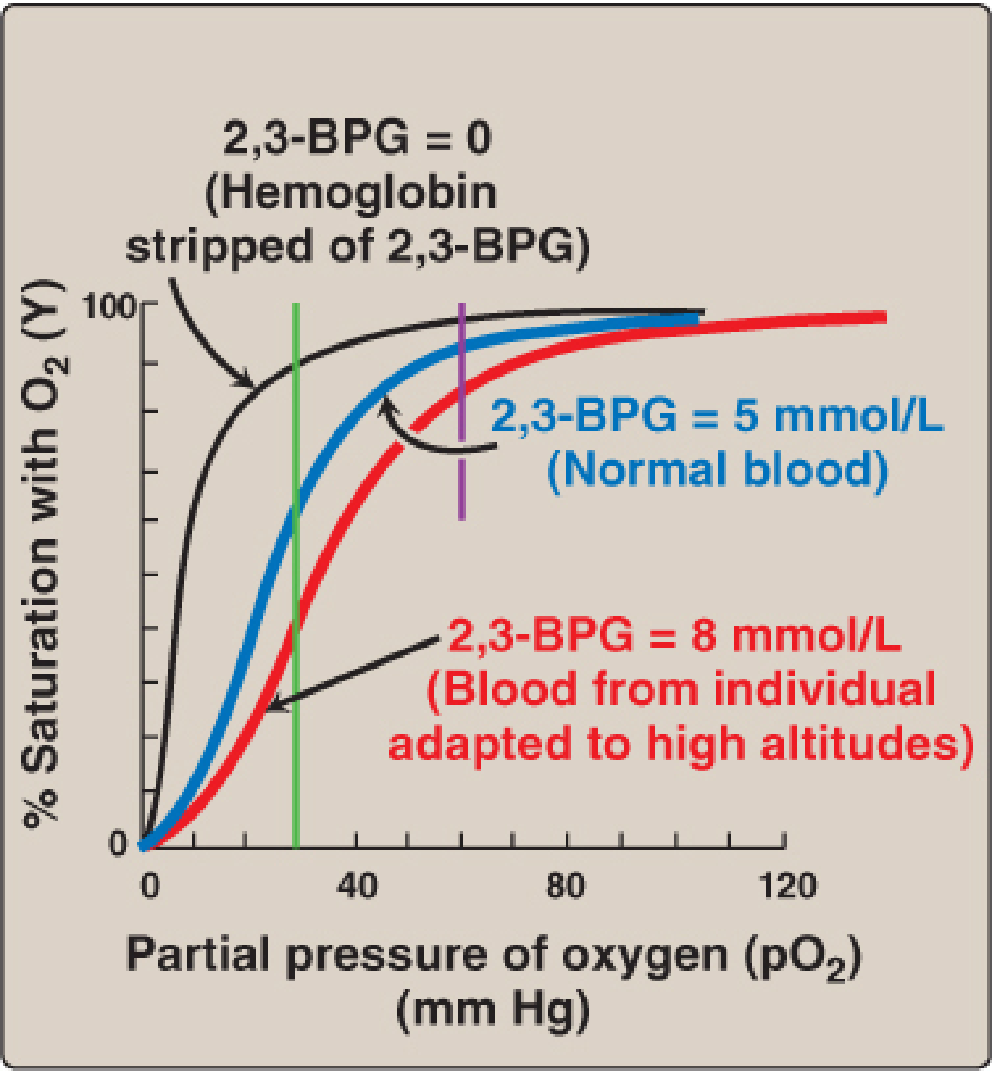
Effect of 2,3-BPG on hemoglobin oxygen affinity. High-altitude adapted blood (red, 2,3-BPG = 8 mmol/L) shows a rightward shift compared to normal blood (blue, 5 mmol/L)

The diagram shows:

Normal blood (blue): 2,3-BPG = 5 mmol/L
High-altitude adapted blood (red): 2,3-BPG = 8 mmol/L - curve is shifted rightward, meaning lower O2 affinity and better tissue oxygen delivery

How the Answer Options Relate

Option	Verdict	Explanation
A. Increase 2,3-BPG	CORRECT (primary)	Chronic hypoxia → ↑ 2,3-BPG synthesis in RBCs
B. Decrease oxygen affinity	CORRECT (consequence)	↑ 2,3-BPG → right shift → ↓ O2 affinity
C. Increase oxygen affinity	Wrong	This is the OPPOSITE; would impair O2 delivery to tissues
D. No change	Wrong	The body actively adapts via this 2,3-BPG mechanism

Exam tip: If forced to pick ONE answer, choose A (Increase 2,3-BPG) as it is the direct biochemical change. "Decrease in oxygen affinity" is the functional consequence. Both A and B together describe the complete adaptive response to high altitude.

When interpreting a capnogram at? 140-Rise in baseline demonstraites hypocarbia Rise in baseline demonstrates rebreathing Rise in height demonstrates expiratory obstruction Slow fall in height demonsitrates expiratory obstruction Slow. rise in height demonstrate inspiratory obstruction

Finding Sources

Searching the Web

capnogram waveform interpretation baseline rise rebreathing slow rise expiratory obstruction

Searching Images

capnogram waveform abnormal patterns rebreathing baseline rise expiratory obstruction

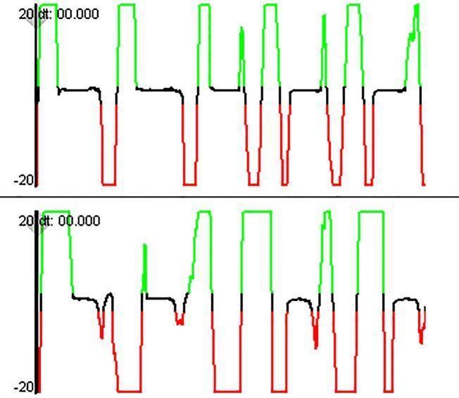
This physiological waveform display illustrates two segments of nasal airflow measurements recorded during 7 seconds of nutritive sucking in an infant. The color-coded waveforms represent distinct respiratory phases: green indicates positive expiratory airflow, red indicates negative inspiratory flow, and black represents transitional or near-zero flow. The top panel (a) demonstrates a pattern with no swallow non-inspiratory flow (SNIF), where the airflow returns to a stable baseline during swallowing events. The bottom panel (b) shows the occurrence of SNIF, visible as distinct, low-amplitude fluctuations in the nasal airflow waveform during the swallowing phase. These measurements, obtained via nasal cannula, are used to evaluate the coordination of breathing and swallowing (the suck-swallow-breathe cycle) and the biomechanical efficiency of infant feeding. The visual data highlights how physiological airflow patterns vary in response to sucking rhythms and swallowing occurrences.

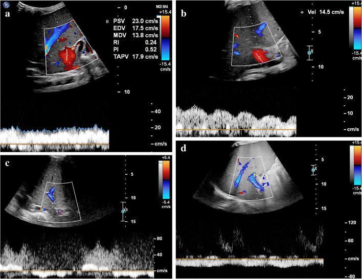
This set of four pediatric axial intercostal color Doppler and spectral ultrasound images demonstrates a spectrum of hepatic portal vein flow patterns associated with Sinusoidal Obstruction Syndrome (SOS). Panel (a) shows normal hepatopetal flow with typical velocity (PSV 23.0 cm/s) and a steady spectral waveform. Panel (b) illustrates increased pulsatility and decreased flow velocity (14.5 cm/s), reflecting rising sinusoidal resistance. Panel (c) displays a 'to-and-fro' pattern, where the spectral waveform alternates between positive and negative deflections, indicating bidirectional, stagnant flow. Panel (d) demonstrates hepatofugal flow, where blood moves away from the liver, appearing as blue signals on Doppler with an inverted spectral waveform below the baseline. These diagnostic images provide critical visual evidence of hemodynamic progression in SOS, ranging from early resistance to advanced portal hypertension and flow reversal. The content is intended for intermediate to advanced medical learners in radiology, hepatology, and pediatric oncology to assist in the classification and monitoring of vascular complications following hematopoietic stem cell transplantation.

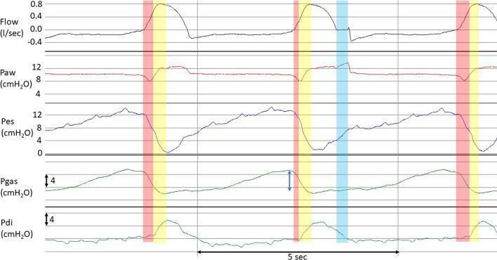
Multi-panel physiological waveform tracing from a patient with Acute Respiratory Distress Syndrome (ARDS) on Proportional Assist Ventilation (PAV+). The diagram displays three respiratory cycles, including an end-inspiratory occluded breath between two unoccluded breaths. The plotted variables include Flow (l/sec), Airway Pressure (Paw), Esophageal Pressure (Pes), Gastric Pressure (Pgas), and Transdiaphragmatic Pressure (Pdi). Color-coded shading highlights phases of muscle activity: red areas indicate initial inspiratory flow generated by expiratory muscle relaxation; yellow areas represent subsequent diaphragmatic contraction; and the blue area marks the end-inspiratory pause (zero flow) during occlusion. Significant expiratory muscle activity is evidenced by a rise in Pgas during expiration (indicated by a blue double-edged arrow). The tracing illustrates how expiratory muscle relaxation contributes to early inspiratory volume and demonstrates the impact of active breathing on transpulmonary driving pressure (ΔPlung) versus respiratory system driving pressure (ΔPrs) calculations. Baseline Pdi returns at the end of the occlusion, indicating a passive state for plateau pressure (Pplat) measurement.

Answer: Rise in baseline demonstrates rebreathing

This is the correct answer. Here is a complete breakdown of the capnogram and all the options:

The Normal Capnogram - 4 Phases

         plateau (Phase III)
       ___________
      /            \
     / Phase II     \ Phase 0
    /  (exp upstroke) \ (insp downstroke)
___/                   \_______________
Phase I (baseline = 0)

Phase	Name	What it represents
Phase I	Inspiratory baseline	Inspired gas - normally CO2 = 0 (zero baseline)
Phase II	Expiratory upstroke	Dead space gas mixing with alveolar gas - rapid rise
Phase III	Alveolar plateau	Alveolar CO2 - nearly flat; peak = EtCO2
Phase 0	Inspiratory downstroke	Start of next breath - CO2 falls back to zero

Analysis of Each Option

✅ Rise in baseline = REBREATHING (CORRECT)

The baseline (Phase I) should be zero - no CO2 during inspiration. If the baseline rises above zero, it means the patient is inhaling CO2 that was not fully cleared from the circuit - this is rebreathing. Causes include:

Exhausted soda lime (in circle breathing circuits)
Faulty inspiratory or expiratory valve
Insufficient fresh gas flow
Increased apparatus dead space

As confirmed by LITFL Capnography Waveform Interpretation: "Elevated inspiratory baseline = CO2 rebreathing (e.g. soda lime exhaustion) or inspiratory valve malfunction."

❌ Rise in baseline = hypocarbia (WRONG)

Hypocarbia (low CO2) would show a decreased HEIGHT (low EtCO2 peak), not a rise in baseline. Hypocarbia → hyperventilation → low EtCO2 value.

❌ Rise in HEIGHT = expiratory obstruction (WRONG - partially misleading)

Rise in height means elevated EtCO2 (hypercarbia/hypoventilation), not specifically expiratory obstruction.
Expiratory obstruction (e.g., bronchospasm) actually causes a slow, sloping rise in Phase II and a prolonged/upward sloping Phase III - the classic "shark fin" pattern - not simply a rise in height.

❌ Slow fall in height = expiratory obstruction (WRONG)

A slow fall (slow Phase 0 downstroke) relates to inspiratory valve malfunction, not expiratory obstruction.

❌ Slow rise in height = inspiratory obstruction (WRONG)

A slow rise in Phase II (the upstroke) with prolonged sloping Phase III = expiratory obstruction (bronchospasm, COPD, kinked tube)
True inspiratory obstruction would affect Phase 0 (the downstroke, not the upstroke)

Key Capnogram Patterns Summary

Abnormal Pattern	Diagnosis
Elevated baseline (doesn't return to 0)	Rebreathing of CO2
Elevated height (high EtCO2)	Hypoventilation / ↑ CO2 production
Low height (low EtCO2)	Hyperventilation / ↓ perfusion / hypocarbia
Slow upstroke + sloping plateau ("shark fin")	Expiratory obstruction (bronchospasm, COPD)
Sudden loss of waveform	ETT dislodgement / disconnection / cardiac arrest
Cleft in plateau	Spontaneous breathing effort against ventilator
Slow downstroke (Phase 0)	Inspiratory valve malfunction

The answer is B - Rise in baseline demonstrates rebreathing. The baseline of a normal capnogram must always return to zero during inspiration; any elevation above zero indicates the patient is breathing in CO2-containing gas (rebreathing).

Create a visual reference chart of capnogram abnormalities

Running Command

mkdir -p /tmp/workspace/capnogram && ls /tmp/workspace/capnogram

Writing File

~/capnogram/capnogram_chart.py

import numpy as np
import matplotlib.pyplot as plt
import matplotlib.patches as mpatches
from matplotlib.patches import FancyArrowPatch
import matplotlib.gridspec as gridspec

# ── colour palette ──────────────────────────────────────────────────────────
BG        = "#0D1B2A"   # deep navy background
PANEL_BG  = "#12263A"   # slightly lighter panel
GRID_COL  = "#1E3A52"
TITLE_COL = "#E8F4FD"
LABEL_COL = "#B0C4D8"
ANNOT_COL = "#FFD166"   # amber annotation
NORMAL_C  = "#06D6A0"   # teal  – normal waveform
ABNORM_C  = "#EF476F"   # rose  – abnormal waveform
ARROW_C   = "#FFD166"
BORDER_C  = "#2A5A7A"

plt.rcParams.update({
    "font.family": "DejaVu Sans",
    "text.color":  LABEL_COL,
    "axes.labelcolor": LABEL_COL,
    "xtick.color": LABEL_COL,
    "ytick.color": LABEL_COL,
})

# ── helper: one capnogram cycle ──────────────────────────────────────────────
def normal_cycle(x_start=0, height=38, baseline=0, n=300):
    """Returns x, y arrays for one normal capnogram cycle."""
    t = np.linspace(0, 1, n)
    y = np.zeros(n)
    # Phase I  – inspiratory baseline  (0–20 %)
    ph1 = int(0.20 * n)
    y[:ph1] = baseline
    # Phase II – expiratory upstroke   (20–35 %)
    ph2 = int(0.35 * n)
    y[ph1:ph2] = baseline + (height - baseline) * (t[ph1:ph2] - t[ph1]) / (t[ph2-1] - t[ph1])
    # Phase III – alveolar plateau     (35–65 %)
    ph3 = int(0.65 * n)
    y[ph2:ph3] = height + np.linspace(0, 1.5, ph3 - ph2)   # tiny upslope
    # Phase 0  – inspiratory downstroke (65–80 %)
    ph4 = int(0.80 * n)
    y[ph3:ph4] = height + 1.5 - (height + 1.5 - baseline) * (t[ph3:ph4] - t[ph3]) / (t[ph4-1] - t[ph3])
    # rest (80–100 %) = baseline
    y[ph4:] = baseline
    x = x_start + t
    return x, y


def slow_upstroke_cycle(x_start=0, height=38, baseline=0, n=300):
    """Shark-fin: slow sloping upstroke + rising plateau – expiratory obstruction."""
    t = np.linspace(0, 1, n)
    y = np.zeros(n)
    ph1 = int(0.20 * n)
    y[:ph1] = baseline
    ph2 = int(0.55 * n)   # upstroke is longer / slower
    y[ph1:ph2] = baseline + (height - baseline) * ((t[ph1:ph2] - t[ph1]) / (t[ph2-1] - t[ph1])) ** 0.6
    ph3 = int(0.72 * n)
    y[ph2:ph3] = height + np.linspace(0, 4, ph3 - ph2)   # steep upward slope
    ph4 = int(0.85 * n)
    y[ph3:ph4] = (height + 4) - (height + 4 - baseline) * (t[ph3:ph4] - t[ph3]) / (t[ph4-1] - t[ph3])
    y[ph4:] = baseline
    x = x_start + t
    return x, y


def rebreathing_cycle(x_start=0, height=38, rise=8, n=300):
    """Baseline does not return to zero."""
    t = np.linspace(0, 1, n)
    y = np.zeros(n)
    ph1 = int(0.20 * n)
    y[:ph1] = rise
    ph2 = int(0.35 * n)
    y[ph1:ph2] = rise + (height - rise) * (t[ph1:ph2] - t[ph1]) / (t[ph2-1] - t[ph1])
    ph3 = int(0.65 * n)
    y[ph2:ph3] = height + np.linspace(0, 1.5, ph3 - ph2)
    ph4 = int(0.78 * n)
    y[ph3:ph4] = (height + 1.5) - ((height + 1.5) - rise) * (t[ph3:ph4] - t[ph3]) / (t[ph4-1] - t[ph3])
    y[ph4:] = rise
    x = x_start + t
    return x, y


def low_height_cycle(x_start=0, height=15, baseline=0, n=300):
    return normal_cycle(x_start, height, baseline, n)


def high_height_cycle(x_start=0, height=60, baseline=0, n=300):
    return normal_cycle(x_start, height, baseline, n)


def cleft_cycle(x_start=0, height=38, n=300):
    """Curare cleft – notch in plateau."""
    x, y = normal_cycle(x_start, height, 0, n)
    mid = int(0.52 * n)
    w = int(0.06 * n)
    for i in range(w):
        frac = np.sin(np.pi * i / w)
        y[mid + i] = height - frac * 12
    return x, y


def gradual_loss_cycles(x_start=0, n=300):
    """Three cycles of progressively falling EtCO2 – waning cardiac output."""
    all_x, all_y = [], []
    for i, h in enumerate([38, 25, 10]):
        x, y = normal_cycle(x_start + i * 1.1, h, 0, n)
        all_x.append(x); all_y.append(y)
    return np.concatenate(all_x), np.concatenate(all_y)


def sudden_loss(x_start=0, n=300):
    """One normal cycle then flat line."""
    x1, y1 = normal_cycle(x_start, 38, 0, n)
    x2 = x_start + np.linspace(1, 2.3, 200)
    y2 = np.zeros(200)
    return np.concatenate([x1, x2]), np.concatenate([y1, y2])


def insp_valve_fault(x_start=0, height=38, n=300):
    """Slow downstroke (Phase 0) – inspiratory valve malfunction."""
    t = np.linspace(0, 1, n)
    y = np.zeros(n)
    ph1 = int(0.20 * n)
    y[:ph1] = 0
    ph2 = int(0.35 * n)
    y[ph1:ph2] = (height) * (t[ph1:ph2] - t[ph1]) / (t[ph2-1] - t[ph1])
    ph3 = int(0.60 * n)
    y[ph2:ph3] = height + np.linspace(0, 1.5, ph3 - ph2)
    ph4 = int(0.95 * n)   # very slow downstroke
    y[ph3:ph4] = (height + 1.5) - (height + 1.5) * (t[ph3:ph4] - t[ph3]) / (t[ph4-1] - t[ph3])
    y[ph4:] = 0
    x = x_start + t
    return x, y


# ── layout ───────────────────────────────────────────────────────────────────
fig = plt.figure(figsize=(20, 26), facecolor=BG)
fig.patch.set_facecolor(BG)

# Title banner
fig.text(0.5, 0.975, "CAPNOGRAM ABNORMALITIES", fontsize=30, fontweight="bold",
         color=TITLE_COL, ha="center", va="top", family="DejaVu Sans")
fig.text(0.5, 0.963, "Visual Reference Chart  |  CO₂ Waveform Interpretation",
         fontsize=14, color=LABEL_COL, ha="center", va="top", style="italic")

# thin horizontal rule under title
ax_rule = fig.add_axes([0.04, 0.956, 0.92, 0.003])
ax_rule.set_facecolor(BORDER_C); ax_rule.axis("off")

# ── grid: 3 columns × 3 rows (+ 1 row for normal reference) ─────────────────
gs = gridspec.GridSpec(4, 3, figure=fig,
                       top=0.950, bottom=0.04,
                       left=0.04, right=0.97,
                       hspace=0.55, wspace=0.28)

# ── helper: style an axis ────────────────────────────────────────────────────
def style_ax(ax, title, color=ABNORM_C, badge=None, badge_color="#EF476F"):
    ax.set_facecolor(PANEL_BG)
    for spine in ax.spines.values():
        spine.set_edgecolor(BORDER_C); spine.set_linewidth(1.2)
    ax.set_xticks([]); ax.set_yticks([])
    ax.set_ylabel("CO₂ (mmHg)", fontsize=9, color=LABEL_COL, labelpad=4)
    ax.set_xlabel("Time →", fontsize=9, color=LABEL_COL, labelpad=2)
    ax.set_title(title, fontsize=12, fontweight="bold", color=color, pad=8)
    ax.axhline(0, color=GRID_COL, linewidth=0.8, linestyle="--")
    if badge:
        ax.text(0.98, 0.96, badge, transform=ax.transAxes,
                fontsize=9, fontweight="bold", color="white",
                ha="right", va="top",
                bbox=dict(boxstyle="round,pad=0.3", facecolor=badge_color, alpha=0.85))

def arrow(ax, x, y, dx, dy, txt, txt_x=None, txt_y=None):
    ax.annotate("", xy=(x+dx, y+dy), xytext=(x, y),
                arrowprops=dict(arrowstyle="->", color=ANNOT_COL, lw=1.5))
    ax.text(txt_x if txt_x else x+dx+0.02, txt_y if txt_y else y+dy,
            txt, fontsize=8, color=ANNOT_COL, va="center")

# ─────────────────────────────────────────────────────────────────────────────
# ROW 0 – NORMAL (spans full width)
# ─────────────────────────────────────────────────────────────────────────────
ax_norm = fig.add_subplot(gs[0, :])
ax_norm.set_facecolor(PANEL_BG)
for spine in ax_norm.spines.values():
    spine.set_edgecolor(BORDER_C); spine.set_linewidth(1.4)
ax_norm.set_xticks([]); ax_norm.set_yticks([])
ax_norm.set_ylabel("CO₂ (mmHg)", fontsize=10, color=LABEL_COL)
ax_norm.set_title("NORMAL CAPNOGRAM  –  Reference", fontsize=14,
                  fontweight="bold", color=NORMAL_C, pad=10)
ax_norm.axhline(0, color=GRID_COL, linewidth=0.8, linestyle="--")

for i in range(3):
    x, y = normal_cycle(i * 1.05, 38)
    ax_norm.plot(x, y, color=NORMAL_C, lw=2.2)

ax_norm.set_xlim(-0.05, 3.25)
ax_norm.set_ylim(-8, 55)

# Phase labels on first cycle
ax_norm.text(0.10, -6,  "I\n(Insp\nbaseline)", fontsize=8, color=ANNOT_COL, ha="center")
ax_norm.text(0.27,  22, "II\n(Exp\nupstroke)", fontsize=8, color=ANNOT_COL, ha="center")
ax_norm.text(0.50,  46, "III\n(Alveolar\nplateau)", fontsize=8, color=ANNOT_COL, ha="center")
ax_norm.text(0.73,  22, "0\n(Insp\ndownstroke)", fontsize=8, color=ANNOT_COL, ha="center")

# EtCO2 brace
ax_norm.annotate("", xy=(0.38, 38), xytext=(0.38, 0),
    arrowprops=dict(arrowstyle="<->", color="#06D6A0", lw=1.5))
ax_norm.text(0.41, 20, "EtCO₂\n35–45 mmHg\n(normal)", fontsize=8.5,
             color=NORMAL_C, va="center")

# Normal badge
ax_norm.text(0.99, 0.97, "NORMAL", transform=ax_norm.transAxes,
             fontsize=10, fontweight="bold", color="white", ha="right", va="top",
             bbox=dict(boxstyle="round,pad=0.35", facecolor=NORMAL_C, alpha=0.9))

# ─────────────────────────────────────────────────────────────────────────────
# ROW 1 – Rebreathing | Expiratory Obstruction | Hypercarbia
# ─────────────────────────────────────────────────────────────────────────────

# 1a  REBREATHING
ax1 = fig.add_subplot(gs[1, 0])
style_ax(ax1, "Elevated Baseline\n(Rebreathing)", badge="REBREATHING", badge_color="#9B5DE5")
for i in range(3):
    x, y = rebreathing_cycle(i * 1.05, height=38, rise=8)
    ax1.plot(x, y, color=ABNORM_C, lw=2.2)
ax1.set_xlim(-0.05, 3.25); ax1.set_ylim(-5, 55)
ax1.axhline(8, color=ANNOT_COL, lw=1, linestyle=":", alpha=0.7)
ax1.text(3.15, 8.5, "↑ baseline\n≠ 0", fontsize=8, color=ANNOT_COL, ha="right")
# causes box
ax1.text(0.02, 0.04,
         "Causes: Exhausted soda lime\nFaulty expiratory valve\nExcess circuit dead space",
         transform=ax1.transAxes, fontsize=7.5, color=LABEL_COL,
         bbox=dict(boxstyle="round,pad=0.4", facecolor=GRID_COL, alpha=0.8))

# 1b  EXPIRATORY OBSTRUCTION (shark fin)
ax2 = fig.add_subplot(gs[1, 1])
style_ax(ax2, "Shark-Fin Pattern\n(Expiratory Obstruction)", badge="EXP. OBSTRUCTION", badge_color="#F77F00")
for i in range(3):
    x, y = slow_upstroke_cycle(i * 1.1, height=42)
    ax2.plot(x, y, color=ABNORM_C, lw=2.2)
ax2.set_xlim(-0.05, 3.5); ax2.set_ylim(-5, 60)
ax2.annotate("Slow sloping\nPhase II+III", xy=(0.42, 25), xytext=(0.65, 10),
             fontsize=8, color=ANNOT_COL,
             arrowprops=dict(arrowstyle="->", color=ANNOT_COL, lw=1.2))
ax2.text(0.02, 0.04,
         "Causes: Bronchospasm / COPD\nKinked ETT / Foreign body\nSevere asthma",
         transform=ax2.transAxes, fontsize=7.5, color=LABEL_COL,
         bbox=dict(boxstyle="round,pad=0.4", facecolor=GRID_COL, alpha=0.8))

# 1c  HYPERCARBIA
ax3 = fig.add_subplot(gs[1, 2])
style_ax(ax3, "Elevated Height\n(Hypercarbia / Hypoventilation)", badge="HIGH EtCO₂", badge_color="#E63946")
for i in range(3):
    x, y = high_height_cycle(i * 1.05, height=62)
    ax3.plot(x, y, color=ABNORM_C, lw=2.2)
# reference normal height dashed
for i in range(3):
    x, y = normal_cycle(i * 1.05, height=38)
    ax3.plot(x, y, color=NORMAL_C, lw=1.2, linestyle="--", alpha=0.5)
ax3.set_xlim(-0.05, 3.25); ax3.set_ylim(-5, 80)
ax3.annotate("EtCO₂ > 45 mmHg", xy=(0.50, 62), xytext=(0.55, 74),
             fontsize=8.5, color=ANNOT_COL,
             arrowprops=dict(arrowstyle="->", color=ANNOT_COL, lw=1.2))
ax3.text(0.02, 0.04,
         "Causes: Hypoventilation\nRespiratory depression\n↑ CO₂ production (fever, sepsis)",
         transform=ax3.transAxes, fontsize=7.5, color=LABEL_COL,
         bbox=dict(boxstyle="round,pad=0.4", facecolor=GRID_COL, alpha=0.8))

# ─────────────────────────────────────────────────────────────────────────────
# ROW 2 – Hypocarbia | Curare Cleft | Inspiratory Valve Fault
# ─────────────────────────────────────────────────────────────────────────────

# 2a  HYPOCARBIA
ax4 = fig.add_subplot(gs[2, 0])
style_ax(ax4, "Low Height\n(Hypocarbia / Hyperventilation)", badge="LOW EtCO₂", badge_color="#118AB2")
for i in range(3):
    x, y = low_height_cycle(i * 1.05, height=15)
    ax4.plot(x, y, color=ABNORM_C, lw=2.2)
for i in range(3):
    x, y = normal_cycle(i * 1.05, height=38)
    ax4.plot(x, y, color=NORMAL_C, lw=1.2, linestyle="--", alpha=0.5)
ax4.set_xlim(-0.05, 3.25); ax4.set_ylim(-5, 55)
ax4.annotate("EtCO₂ < 35 mmHg", xy=(0.50, 15), xytext=(0.60, 28),
             fontsize=8.5, color=ANNOT_COL,
             arrowprops=dict(arrowstyle="->", color=ANNOT_COL, lw=1.2))
ax4.text(0.02, 0.04,
         "Causes: Hyperventilation\nPulmonary embolism\nHypovolaemia / Low cardiac output",
         transform=ax4.transAxes, fontsize=7.5, color=LABEL_COL,
         bbox=dict(boxstyle="round,pad=0.4", facecolor=GRID_COL, alpha=0.8))

# 2b  CURARE CLEFT
ax5 = fig.add_subplot(gs[2, 1])
style_ax(ax5, "Curare Cleft / Notch\n(Spontaneous Breathing Effort)", badge="CURARE CLEFT", badge_color="#7B2D8B")
for i in range(3):
    x, y = cleft_cycle(i * 1.05, height=38)
    ax5.plot(x, y, color=ABNORM_C, lw=2.2)
ax5.set_xlim(-0.05, 3.25); ax5.set_ylim(-5, 55)
ax5.annotate("Notch in plateau\n(patient breathing\nagainst ventilator)", xy=(0.52, 26), xytext=(0.60, 8),
             fontsize=8, color=ANNOT_COL,
             arrowprops=dict(arrowstyle="->", color=ANNOT_COL, lw=1.2))
ax5.text(0.02, 0.04,
         "Causes: Residual neuromuscular block\nLight anaesthesia\nSpontaneous inspiratory effort",
         transform=ax5.transAxes, fontsize=7.5, color=LABEL_COL,
         bbox=dict(boxstyle="round,pad=0.4", facecolor=GRID_COL, alpha=0.8))

# 2c  INSPIRATORY VALVE MALFUNCTION
ax6 = fig.add_subplot(gs[2, 2])
style_ax(ax6, "Slow Downstroke\n(Inspiratory Valve Malfunction)", badge="INSP. VALVE FAULT", badge_color="#2D6A4F")
for i in range(3):
    x, y = insp_valve_fault(i * 1.05, height=38)
    ax6.plot(x, y, color=ABNORM_C, lw=2.2)
ax6.set_xlim(-0.05, 3.25); ax6.set_ylim(-5, 55)
ax6.annotate("Prolonged\ndownstroke\n(Phase 0)", xy=(0.77, 18), xytext=(0.82, 36),
             fontsize=8, color=ANNOT_COL,
             arrowprops=dict(arrowstyle="->", color=ANNOT_COL, lw=1.2))
ax6.text(0.02, 0.04,
         "Causes: Sticky inspiratory valve\nCircuit leak\nPartially obstructed inspiratory limb",
         transform=ax6.transAxes, fontsize=7.5, color=LABEL_COL,
         bbox=dict(boxstyle="round,pad=0.4", facecolor=GRID_COL, alpha=0.8))

# ─────────────────────────────────────────────────────────────────────────────
# ROW 3 – Sudden Loss | Gradual Decline | Cardiac Oscillations
# ─────────────────────────────────────────────────────────────────────────────

# 3a  SUDDEN LOSS
ax7 = fig.add_subplot(gs[3, 0])
style_ax(ax7, "Sudden Loss of Waveform\n(ETT Dislodgement / Cardiac Arrest)", badge="SUDDEN LOSS", badge_color="#D62828")
x, y = sudden_loss(0)
ax7.plot(x, y, color=ABNORM_C, lw=2.2)
ax7.set_xlim(-0.05, 2.4); ax7.set_ylim(-5, 55)
ax7.annotate("Waveform absent\nafter this point", xy=(1.10, 1), xytext=(1.15, 20),
             fontsize=8, color=ANNOT_COL,
             arrowprops=dict(arrowstyle="->", color=ANNOT_COL, lw=1.2))
ax7.text(0.02, 0.04,
         "Causes: ETT dislodged / oesophageal\nintubation / circuit disconnect\nCardiac arrest (no perfusion)",
         transform=ax7.transAxes, fontsize=7.5, color=LABEL_COL,
         bbox=dict(boxstyle="round,pad=0.4", facecolor=GRID_COL, alpha=0.8))

# 3b  GRADUAL DECLINE
ax8 = fig.add_subplot(gs[3, 1])
style_ax(ax8, "Gradual Decline in EtCO₂\n(Decreasing Cardiac Output / PE)", badge="GRADUAL DROP", badge_color="#F4A261")
x, y = gradual_loss_cycles(0)
ax8.plot(x, y, color=ABNORM_C, lw=2.2)
ax8.set_xlim(-0.05, 3.6); ax8.set_ylim(-5, 55)
ax8.annotate("Progressive\ndrop in EtCO₂", xy=(2.2, 10), xytext=(2.3, 28),
             fontsize=8, color=ANNOT_COL,
             arrowprops=dict(arrowstyle="->", color=ANNOT_COL, lw=1.2))
ax8.text(0.02, 0.04,
         "Causes: Pulmonary embolism\nHaemorrhage / hypovolaemia\nWorsening cardiac output",
         transform=ax8.transAxes, fontsize=7.5, color=LABEL_COL,
         bbox=dict(boxstyle="round,pad=0.4", facecolor=GRID_COL, alpha=0.8))

# 3c  CARDIAC OSCILLATIONS (small waves on baseline)
ax9 = fig.add_subplot(gs[3, 2])
style_ax(ax9, "Cardiac Oscillations\n(Small Ripples on Waveform)", badge="CARDIAC OSCILLATIONS", badge_color="#457B9D")
# simulate: normal cycles with small sinusoidal ripples on plateau
for i in range(3):
    x, y = normal_cycle(i * 1.05, height=38)
    # add cardiac oscillations on plateau portion
    osc_mask = (x - i*1.05 > 0.35) & (x - i*1.05 < 0.65)
    x_osc = x[osc_mask] - i*1.05
    y[osc_mask] += 3.5 * np.sin(40 * np.pi * x_osc)
    ax9.plot(x, y, color=ABNORM_C, lw=2.0)
ax9.set_xlim(-0.05, 3.25); ax9.set_ylim(-5, 55)
ax9.annotate("Ripples on\nplateau", xy=(0.51, 42), xytext=(0.60, 50),
             fontsize=8, color=ANNOT_COL,
             arrowprops=dict(arrowstyle="->", color=ANNOT_COL, lw=1.2))
ax9.text(0.02, 0.04,
         "Causes: Cardiac pulsations transmitted\nto airway (especially in small patients)\nUsually benign finding",
         transform=ax9.transAxes, fontsize=7.5, color=LABEL_COL,
         bbox=dict(boxstyle="round,pad=0.4", facecolor=GRID_COL, alpha=0.8))

# ── legend strip at bottom ───────────────────────────────────────────────────
legend_ax = fig.add_axes([0.04, 0.012, 0.92, 0.022])
legend_ax.set_facecolor(PANEL_BG); legend_ax.axis("off")
legend_ax.plot([0.01, 0.045], [0.5, 0.5], color=NORMAL_C, lw=2.5, transform=legend_ax.transAxes)
legend_ax.text(0.05, 0.5, "Normal (reference)", color=NORMAL_C, fontsize=9,
               va="center", transform=legend_ax.transAxes)
legend_ax.plot([0.25, 0.285], [0.5, 0.5], color=ABNORM_C, lw=2.5, transform=legend_ax.transAxes)
legend_ax.text(0.295, 0.5, "Abnormal waveform", color=ABNORM_C, fontsize=9,
               va="center", transform=legend_ax.transAxes)
legend_ax.text(0.99, 0.5,
               "EtCO₂ normal range: 35–45 mmHg  |  Baseline should always = 0  |  Shape = square wave",
               color=LABEL_COL, fontsize=8.5, va="center", ha="right", transform=legend_ax.transAxes)

plt.savefig("/tmp/workspace/capnogram/capnogram_abnormalities.png",
            dpi=180, bbox_inches="tight", facecolor=BG)
print("Saved.")

Running Command

cd /tmp/workspace/capnogram && python capnogram_chart.py 2>&1

Here is your visual reference chart:

capnogram abnormalities

Image · PNG

The chart covers 9 capnogram patterns arranged across 4 rows:

Row 1 - Normal Reference (full width)

Phase I (inspiratory baseline = 0), Phase II (expiratory upstroke), Phase III (alveolar plateau), Phase 0 (inspiratory downstroke) - all labelled with EtCO2 normal range of 35-45 mmHg

Row 2 - Three core abnormalities

Elevated Baseline - rebreathing (soda lime exhaustion, faulty valves)
Shark-Fin Pattern - expiratory obstruction (bronchospasm, COPD)
Elevated Height - hypercarbia/hypoventilation

Row 3 - Three more patterns

Low Height - hypocarbia/hyperventilation (with normal dashed for comparison)
Curare Cleft - notch in plateau from spontaneous breathing effort against ventilator
Slow Downstroke - inspiratory valve malfunction

Row 4 - Critical patterns

Sudden Loss - ETT dislodgement, oesophageal intubation, cardiac arrest
Gradual Decline - decreasing cardiac output, pulmonary embolism, haemorrhage
Cardiac Oscillations - benign ripples from cardiac pulsations transmitted to airway

Each panel includes the pattern name, a colour-coded badge, and a causes box at the bottom.

Hypoxemia in blood is sensed by: Chemoreccptors Central receptors carotid sinus

Finding Sources

Reading File

Answer: Chemoreceptors - specifically Peripheral Chemoreceptors (Carotid Bodies)

The correct answer is Chemoreceptors - but the critical distinction to know for the exam is which type senses hypoxemia, and why the other options are wrong.

The Two Types of Chemoreceptors

Feature	Peripheral Chemoreceptors	Central Chemoreceptors
Location	Carotid bodies (bifurcation of carotid artery) + Aortic bodies (aortic arch)	Retrotrapezoid nucleus (RTN), medulla oblongata
Primary stimulus	↓ PaO2 (hypoxemia)	↑ PaCO2 / ↓ pH (NOT O2)
Also respond to	↑ PaCO2, ↓ pH, ↑ temperature	Extracellular pH changes
Speed	Rapid / acute changes	Steady-state / chronic
O2 sensing	YES - primary sensor	NO

Why Peripheral Chemoreceptors (Carotid Bodies) Sense Hypoxemia

Directly from Fishman's Pulmonary Diseases & Disorders:

"Peripheral chemoreceptors are sensory cells in the arterial circulation that monitor the environment outside of the CNS for changes in pH, O2, and CO2... The carotid bodies receive the highest blood flow rate of any organ in the body, which allows for nearly continuous sensing of changes in arterial oxygen (PaO2)... Carotid bodies are most sensitive to changes in PaO2."

The carotid body contains type I (glomus) cells that act as oxygen sensors. When PaO2 falls, they release neurotransmitters that activate the glossopharyngeal nerve (CN IX), sending signals to the respiratory centre in the brainstem to increase ventilation.

Why Central Chemoreceptors Do NOT Sense Hypoxemia

Central chemoreceptors in the medulla are surrounded by the blood-brain barrier, which:

Is impermeable to H⁺ ions from the blood
Responds to CO2 diffusing across and generating H⁺ in the CSF
Cannot detect changes in blood PaO2 directly

Therefore, central receptors sense hypercapnia (↑ CO2), not hypoxemia.

Why "Carotid Sinus" is Wrong

The carotid sinus is a baroreceptor, NOT a chemoreceptor:

Located at the bifurcation of the common carotid artery
Senses arterial blood pressure (stretch), not oxygen
Signals via CN IX to regulate heart rate and BP (baroreflex)

The carotid body (nearby but distinct) is the chemoreceptor that senses O2.

Summary Flow

↓ PaO2 (hypoxemia)
        ↓
Carotid body type I (glomus) cells activated
        ↓
CN IX → Nucleus tractus solitarius (NTS) → Respiratory centre
        ↓
↑ Respiratory rate + ↑ Tidal volume
        ↓
↑ Alveolar ventilation → PaO2 restored

Answer: Chemoreceptors (peripheral - carotid bodies) sense hypoxemia in blood. Central chemoreceptors sense CO2/pH. The carotid sinus is a baroreceptor and does not sense oxygen. - Fishman's Pulmonary Diseases and Disorders

A pt presented with paralysis of leg and aphasia .. artery involved?

Finding Sources

Searching Images

anterior cerebral artery territory stroke leg paralysis cortical homunculus

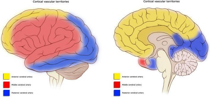
This anatomical diagram illustrates the cortical vascular territories of the human brain through lateral (left) and midsagittal (right) views. The territories are color-coded to differentiate the areas supplied by the three major cerebral arteries. The Anterior Cerebral Artery (ACA) territory, highlighted in yellow, encompasses the medial surface of the frontal and parietal lobes, extending to the superior border of the lateral surface. The Middle Cerebral Artery (MCA) territory, shown in red, dominates the lateral surface, covering the majority of the frontal, parietal, and temporal lobes, including the primary motor and sensory cortices. The Posterior Cerebral Artery (PCA) territory, marked in blue, supplies the occipital lobe, the inferior portion of the temporal lobe, and the posterior medial surface. The diagram serves as a clinical education tool for understanding stroke syndromes and neuroanatomical localization, highlighting the watershed zones where these arterial territories meet. Key structures visible include the cerebral cortex, cerebellum, and brainstem.

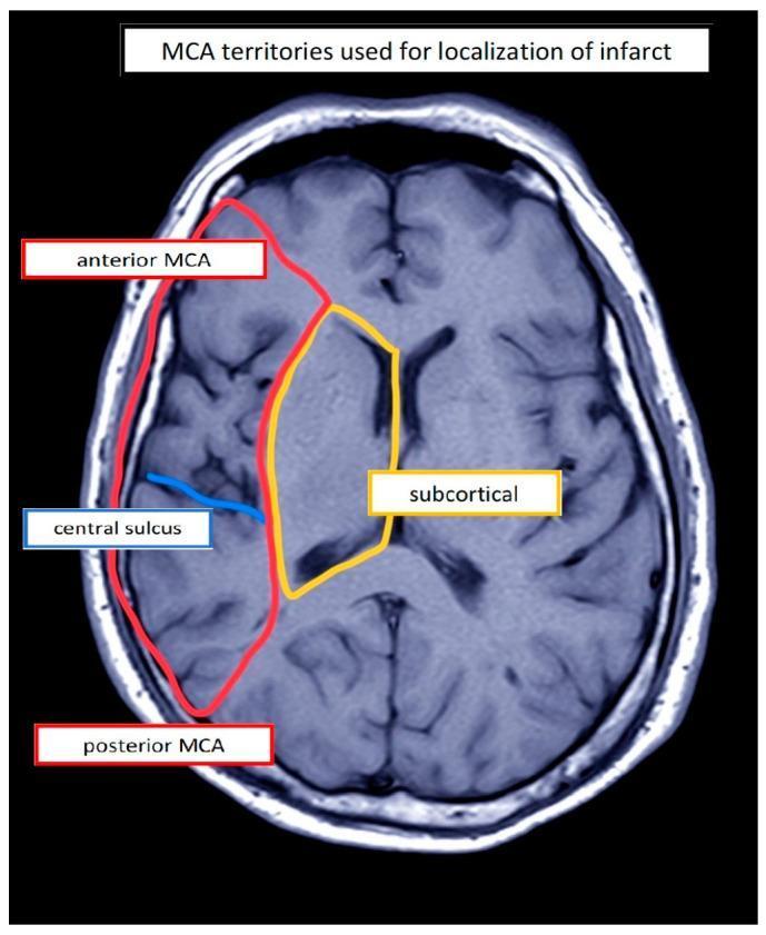
This diagnostic image is a transverse axial section of a brain MRI, utilized to demonstrate Middle Cerebral Artery (MCA) territories for infarct localization. The image displays the cerebral hemispheres with clearly defined cortical gyri and sulci. Colored overlays delineate specific neuroanatomical regions in the left hemisphere: two red-outlined areas identify the anterior MCA territory (frontal region) and the posterior MCA territory (parietal/temporal region). These cortical territories are separated by a blue line marking the central sulcus. A yellow-outlined region indicates the deeper subcortical territory, encompassing the basal ganglia and internal capsule regions. The image serves as an educational tool for stroke neurology and neuroradiology, illustrating the vascular distribution of the MCA and the anatomical landmarks used to categorize ischemic lesions. Such classification is clinically relevant for assessing stroke severity and predicting functional outcomes, such as aphasia or motor deficits.

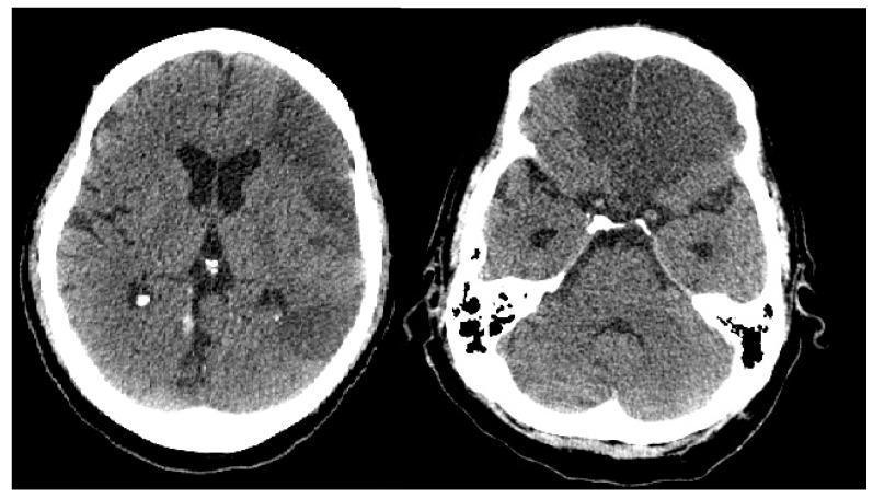
Two non-contrast axial CT images of the brain demonstrate a massive ischemic stroke. There is a prominent, well-demarcated area of hypoattenuation (decreased density) affecting the territory of the left middle cerebral artery and bilateral anterior cerebral arteries. Key anatomical features include a loss of gray-white matter differentiation and effacement of the cortical sulci in the affected regions, indicating significant cytotoxic edema. The ventricles are visible, though the left lateral ventricle shows signs of subtle compression due to the mass effect from the extensive infarction. The right hemisphere maintains relatively normal parenchymal density for comparison. This diagnostic imaging highlights the typical radiologic progression of a large-vessel occlusion and subsequent cerebral ischemia, essential for understanding vascular neurology and emergency stroke management.

Finding Sources

Reading File

Finding Sources

Reading File

Loading Image

Answer: Anterior Cerebral Artery (ACA)

Why ACA?

The key to this question is understanding the somatotopic organisation of the motor cortex (homunculus):

The leg/foot area of the motor cortex sits on the medial surface of the cerebral hemisphere, in the paracentral lobule
The ACA is the only major cerebral artery that supplies the medial surface of the frontal and parietal lobes
Aphasia occurs when the dominant (left) hemisphere ACA territory is infarcted, affecting the supplementary motor area and medial frontal speech regions

This is confirmed directly by Harrison's Principles of Internal Medicine:

"Paralysis of opposite foot and leg: Motor leg area [ACA territory]"

Harrison's Principles of Internal Medicine 22E

ACA Territory - Medial Brain Diagram (Harrison's)

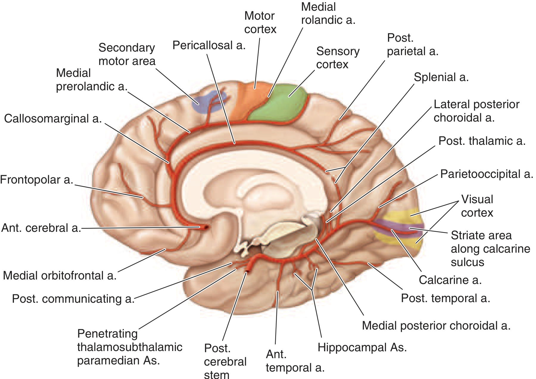
Medial view of cerebral hemisphere showing ACA distribution - the anterior cerebral artery (Ant. cerebral a.) and its branches supply the motor cortex for the leg on the medial surface

Note the Ant. cerebral a. supplying the medial motor cortex (orange area) where the leg representation sits.

Complete ACA Syndrome

Feature	Structure Involved
Contralateral leg/foot paralysis	Motor leg area (paracentral lobule)
Lesser arm paresis	Arm area of cortex / corona radiata
Cortical sensory loss in foot/leg	Sensory area for foot and leg
Urinary incontinence	Sensorimotor area in paracentral lobule
Aphasia (if dominant hemisphere)	Supplementary motor area / medial frontal
Grasp reflex, gegenhalten	Medial posterior frontal lobe
Gait apraxia	Frontal cortex near leg motor area
Abulia / akinetic mutism	Cingulate gyrus / medial frontal

Why NOT Middle Cerebral Artery (MCA)?

This is the most common exam trap. Here is how to distinguish:

Feature	ACA	MCA
Leg weakness	Severe (predominant)	Mild (face > arm > leg)
Arm weakness	Mild	Severe
Face weakness	None	Yes
Aphasia	Possible (supplementary motor area)	Yes (Broca/Wernicke)
Cortical territory	Medial surface	Lateral surface

The classic MCA stroke = face + arm weakness > leg, with aphasia (if dominant) - the leg is SPARED relative to the arm/face because the MCA does not supply the medial leg area.

In this question, leg paralysis is the dominant feature + aphasia = ACA of the dominant hemisphere.

Vascular territory map

Cortical vascular territories - ACA (yellow, medial) supplies leg area; MCA (red, lateral) supplies arm/face; PCA (blue) supplies occipital lobe

Answer: Anterior Cerebral Artery (ACA) - supplies the medial motor cortex (leg area) and, when the dominant hemisphere is involved, causes aphasia via supplementary motor area infarction.

This is a shared conversation. Sign in to Orris to start your own chat.