
cardiac muscle mechanics and the ventricle in details
cardiac muscle excitation contraction coupling sarcomere diagram
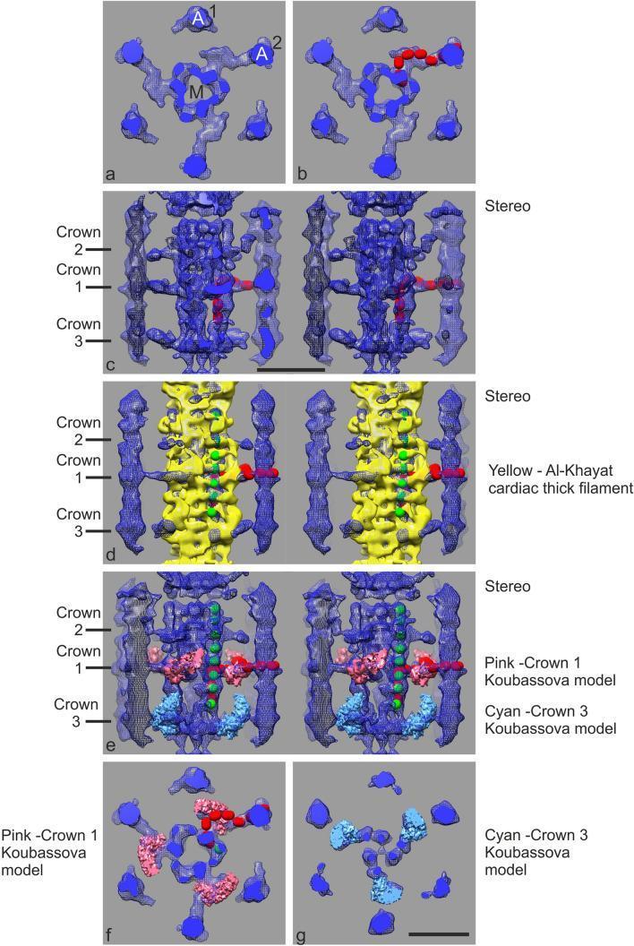
A multi-panel scientific visualization showing subtomogram averages and molecular docking models of the cardiac muscle sarcomere's C-zone, specifically focusing on the interactions between myosin thick filaments and actin thin filaments. Panel (a) provides a cross-sectional view of a central myosin filament (M) surrounded by six actin filaments (A1, A2), illustrating the threefold symmetry of the thick filament backbone. Panels (b-g) integrate structural models to characterize MyBP-C (myosin-binding protein C) and myosin head arrangements. Longitudinal stereo views (c-e) demonstrate the axial distribution of myosin crossbridge 'crowns' (Crowns 1, 2, and 3) along the 430 Å repeat, with Crown 1 coinciding with the MyBP-C stripe. The models incorporate Ig-domain spheres (red) to trace the path of MyBP-C from the myosin backbone to actin, alongside docked crystal structures of cardiac thick filaments (yellow) and myosin motor domains (pink/cyan). This diagram serves as a high-resolution anatomical and physiological illustration for understanding cardiac muscle contraction at the molecular level, highlighting the spatial relationship between titin, MyBP-C, and the actomyosin complex.
![This physiological diagram illustrates simulated calcium dynamics in rat ventricular myocytes, focusing on the mechanisms of excitation-contraction coupling. The image is divided into five panels (A-E) tracking parameters over a 1.0-second timeline. Panel A (Ca2+ sparks) shows high-amplitude calcium spikes in the dyadic subspace ([Ca2+]ds) reaching ~100 µM. Panel B (Ca2+ quarks) displays lower-amplitude, high-frequency [Ca2+]ds fluctuations below 10 µM, representing 'invisible' leak events. Panel C tracks the dynamics of junctional sarcoplasmic reticulum (jSR) calcium release ([Ca2+]jsr), demonstrating local depletion following release events. Panel D quantifies the number of Ryanodine Receptor (RyR) openings, ranging from 0 to 50. Panel E illustrates the concentration of calcium-bound calmodulin complex ([CaCm2+]ds). These charts demonstrate the stochastic nature of calcium release units (CRUs) and the correlation between RyR channel opening and subspace calcium elevation. The data is relevant to cardiac electrophysiology, specifically the study of cardiac alternans and intracellular calcium signaling in cardiomyocytes.](https://cdn.orris.care/cdss_images/pmc_clinical_VQA_79b4efe7519feda5ae5e3f2a613f9970132beae439a1d7f553d9ac4973bb6d97.jpg)
This physiological diagram illustrates simulated calcium dynamics in rat ventricular myocytes, focusing on the mechanisms of excitation-contraction coupling. The image is divided into five panels (A-E) tracking parameters over a 1.0-second timeline. Panel A (Ca2+ sparks) shows high-amplitude calcium spikes in the dyadic subspace ([Ca2+]ds) reaching ~100 µM. Panel B (Ca2+ quarks) displays lower-amplitude, high-frequency [Ca2+]ds fluctuations below 10 µM, representing 'invisible' leak events. Panel C tracks the dynamics of junctional sarcoplasmic reticulum (jSR) calcium release ([Ca2+]jsr), demonstrating local depletion following release events. Panel D quantifies the number of Ryanodine Receptor (RyR) openings, ranging from 0 to 50. Panel E illustrates the concentration of calcium-bound calmodulin complex ([CaCm2+]ds). These charts demonstrate the stochastic nature of calcium release units (CRUs) and the correlation between RyR channel opening and subspace calcium elevation. The data is relevant to cardiac electrophysiology, specifically the study of cardiac alternans and intracellular calcium signaling in cardiomyocytes.
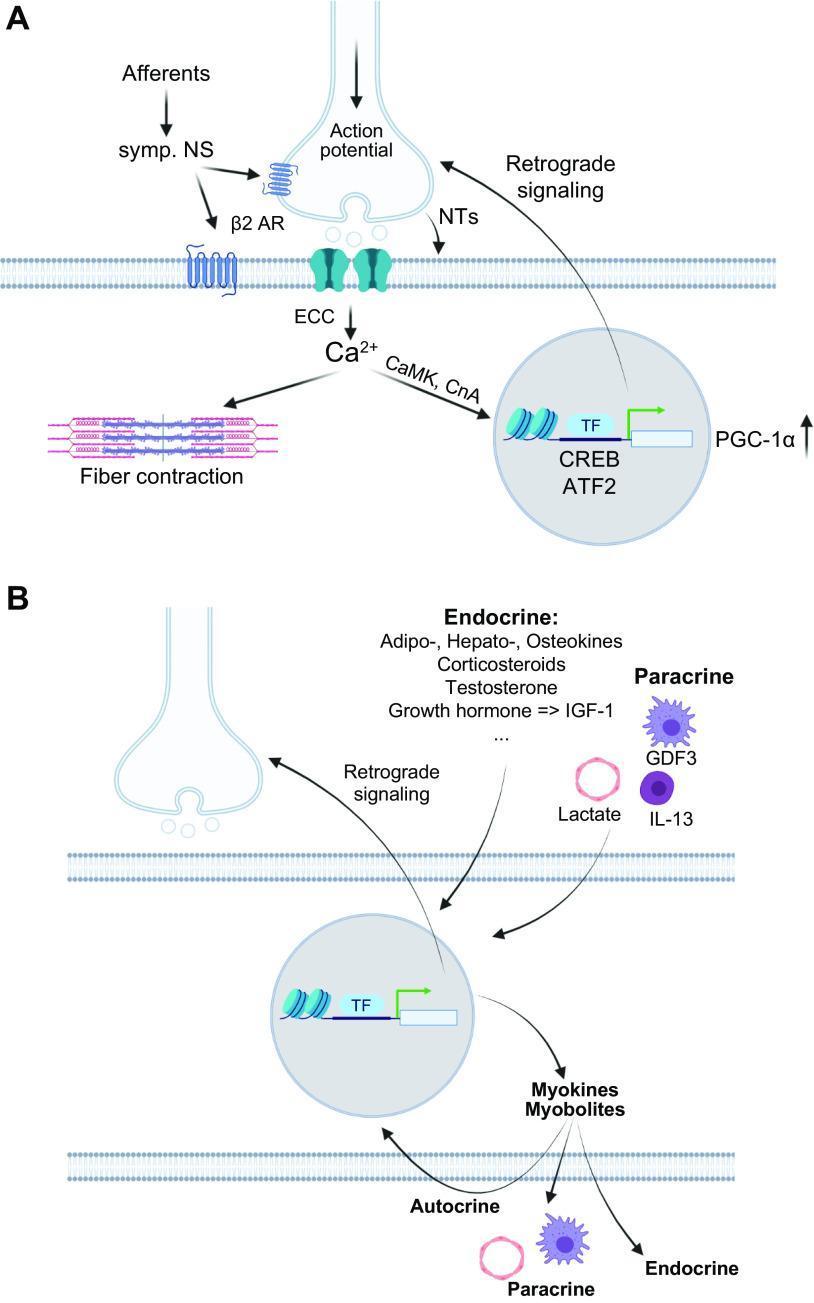
A two-panel (A and B) pathophysiology diagram illustrating motor neuron signaling, excitation-contraction coupling (ECC), and (neuro)endocrine skeletal muscle responses. Panel A depicts the neuromuscular junction where an action potential triggers ECC and the release of intramyocellular calcium (Ca2+), leading to myofiber contraction. It also shows Ca2+ activating signaling pathways (CaMK, CnA) that modulate transcriptional factors (CREB, ATF2) and the coactivator PGC-1̑ in the nucleus, alongside retrograde feedback to the motor neuron via neurotrophic factors (NTs). Adrenergic signaling through ̒2-adrenoreceptors (̒2 AR) from the sympathetic nervous system is also represented. Panel B focuses on 'exerkines,' showing the secretion of myokines and myobolites from the muscle cell. It classifies signaling effects as autocrine, paracrine (e.g., GDF3, IL-13, Lactate), and endocrine. Endocrine factors listed include adipokines, hepatokines, osteokines, corticosteroids, testosterone, and growth hormone-regulated IGF-1, highlighting the systemic coordination between muscle, liver, adipose, and bone tissues during contractile activity.
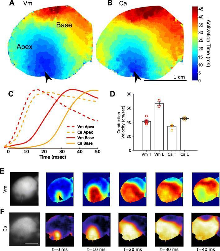
This composite educational graphic illustrates multiparametric optical mapping of cardiac excitation-contraction coupling in an isolated heart model. Panels A and B present isochronal activation maps for transmembrane voltage (Vm) and intracellular calcium (Ca), respectively, showing impulse propagation from the apex (blue) to the base (red) over a 45 ms scale. Panel C displays representative signal upstroke traces, highlighting the physiological lag between electrical depolarization (Vm) and calcium release (Ca) at both the apex and base. Panel D provides a bar chart comparing transverse (T) and longitudinal (L) conduction velocities for Vm and Ca, indicating significantly faster longitudinal Vm propagation compared to Ca. Panels E and F show sequential time-lapse frames (t=0 to 40 ms) of wavefront propagation following electrical pacing at the apex (indicated by arrows). These frames demonstrate the development of spatial heterogeneity and wavebreak in the calcium channel at t=40 ms, serving as a model for studying electrophysiological discontinuities and potential arrhythmogenic precursors.
ventricular pressure volume loop cardiac cycle diastole systole
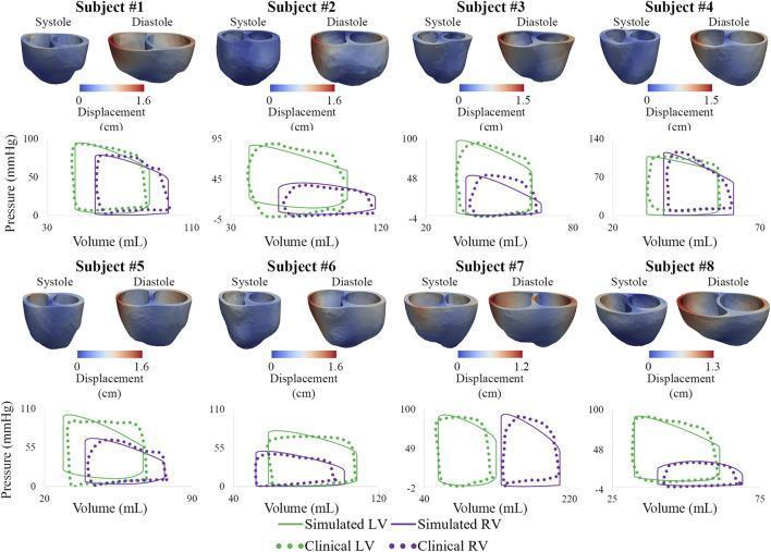
This medical graphic presents a multi-subject comparative study (8 subjects) of cardiovascular mechanics, combining biventricular displacement maps and pressure-volume (PV) loops. The top portion of each subject panel shows 3D color-coded ventricular models during end-systole and end-diastole. Displacement is mapped on a scale from 0 cm (blue) to approximately 1.2–1.6 cm (red), illustrating wall motion across the cardiac cycle. Below each set of models, PV loops represent ventricular hemodynamics. These loops compare left ventricle (LV, green) and right ventricle (RV, purple) data. Solid lines represent computational simulations, while dotted lines represent clinical measurements. The data demonstrates the relationship between pressure (mmHg) and volume (mL), facilitating an assessment of contractility, ejection fraction, and stroke work. The variety in loop morphology and displacement patterns across the subjects highlights patient-specific pathological states, likely in the context of Pulmonary Arterial Hypertension (PAH), where RV remodeling and displacement abnormalities are clinically significant.
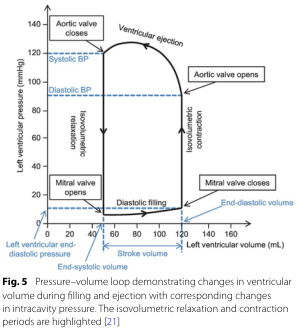
Summary : This figure shows a pressure–volume loop for the left ventricle, illustrating how ventricular volume and pressure change during the cardiac cycle, with key phases and valve events annotated. The isovolumetric relaxation and contraction periods are highlighted, and systolic/diastolic blood pressures are marked. pressure–volume loop diagram: # Title & Axes : • No explicit title on the figure, but the legend describes it as a "Pressure–volume loop demonstrating changes in ventricular volume during filling and ejection with corresponding changes in intracavity pressure." • X-axis: "Left ventricular volume (mL)" with tick marks at 0, 20, 40, 60, 80, 100, 120, 140, 160. • Y-axis: "Left ventricular pressure (mmHg)" with tick marks at 0, 20, 40, 60, 80, 100, 120, 140. • Additional axis labels: "Left ventricular end-diastolic pressure" (blue, left), "End-diastolic volume" (blue, bottom right), "Stroke volume" (black, bottom center). # Phases & Events : • Isovolumetric relaxation: vertical line at low volume, pressure drops, labeled. • Diastolic filling: horizontal line at low pressure, volume increases, labeled. • Isovolumetric contraction: vertical line at high volume, pressure rises, labeled. • Ventricular ejection: curved line, volume decreases as pressure peaks and falls, labeled. • Valve events: – Mitral valve opens (bottom left corner, low pressure/volume). – Mitral valve closes (bottom right corner, high volume/low pressure). – Aortic valve opens (top right corner, high volume/high pressure). – Aortic valve closes (top left corner, low volume/high pressure). # Blood Pressure Markers : • Systolic BP: horizontal dashed blue line at ~120 mmHg. • Diastolic BP: horizontal dashed blue line at ~80 mmHg. # Design Encodings : • Black solid lines for the loop. • Blue dashed lines for blood pressure markers. • Blue text for end-diastolic volume/pressure. • Labeled arrows for direction of phases and valve events. # Analysis : • The loop traces the cardiac cycle, starting at low pressure/volume (end-systolic), filling during diastole, rising sharply during isovolumetric contraction, ejecting blood during ventricular ejection, and dropping pressure during isovolumetric relaxation. • Systolic and diastolic blood pressures are marked, showing the pressure range during ejection. • The width of the loop (horizontal distance) represents stroke volume. • The figure clearly distinguishes the four main phases and the timing of valve openings/closings, providing a comprehensive view of ventricular mechanics during a heartbeat.
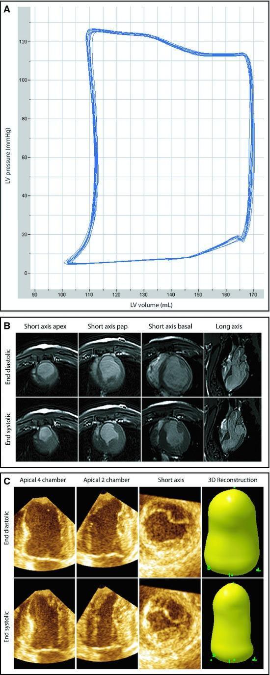
Educational composite figure demonstrating multimodal assessment of left ventricular (LV) function and volume. Panel A shows a Pressure-Volume (PV) loop graph plotting LV pressure (mmHg) against LV volume (mL), characteristic of cardiac cycle analysis. Panel B displays Cardiac Magnetic Resonance Imaging (CMRI) in a 2x4 grid comparing end-diastolic and end-systolic phases across four planes: short-axis apex, papillary muscle level, basal level, and long-axis view. These views highlight ventricular wall thickening and chamber reduction during systole. Panel C illustrates Three-Dimensional Echocardiography (3DE) including apical 4-chamber, apical 2-chamber, and short-axis views alongside a computed 3D reconstruction of the LV volume. The contrast between end-diastolic and end-systolic frames in both CMRI and 3DE allows for the calculation of stroke volume and ejection fraction. The figure serves as a comparative reference for diagnostic imaging modalities used in cardiology to quantify cardiac remodeling and performance after myocardial injury.
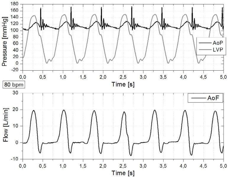
This physiological waveform graph displays cardiac simulator signals at a heart rate of 80 bpm, illustrating hemodynamic relationships across the cardiac cycle over a 5-second interval. The upper panel tracks Pressure (mmHg), comparing Left Ventricular Pressure (LVP) and Aortic Pressure (AoP). The LVP waveform shows cyclical rises to approximately 150 mmHg during systole, falling near 0 mmHg in diastole. The AoP oscillates between roughly 105 and 130 mmHg, with distinct high-frequency spikes (dicrotic notches/oscillations) occurring at the moment of mechanical aortic valve closure. The lower panel displays Aortic Root Flow (AoF) in L/min, showing pulsatile flow synchronized with pressure changes. Flow peaks at approximately 20 L/min during the rapid ejection phase and exhibits a brief negative deflection (backflow) to roughly -8 L/min, indicating closure of the aortic valve. These waveforms serve as a diagnostic algorithm illustration for understanding the relationship between chamber pressure, arterial pressure, and forward stroke volume in cardiovascular physiology.
Cardiac Muscle Mechanics and the Ventricle
1. Cardiac Muscle Cell Structure
- Sarcomeres run from Z line to Z line and contain thick filaments (myosin) and thin filaments (actin + tropomyosin + troponin). The myosin globular heads carry both actin-binding sites and ATPase activity. Troponin C binds Ca²⁺; troponin I is the inhibitory subunit; troponin T anchors the complex to tropomyosin.
- T tubules invaginate at the Z lines (not at the A-I junction as in skeletal muscle) and carry action potentials into the cell interior. They form dyads (not triads) with the sarcoplasmic reticulum (SR).
- The SR is both a Ca²⁺ storage site and a release site, tightly coupled to the T tubule for excitation-contraction coupling.
- Cardiac myocytes are connected end-to-end via intercalated discs containing gap junctions, which allow rapid electrical coupling so the heart behaves as a functional syncytium.
2. Excitation-Contraction Coupling (ECC)
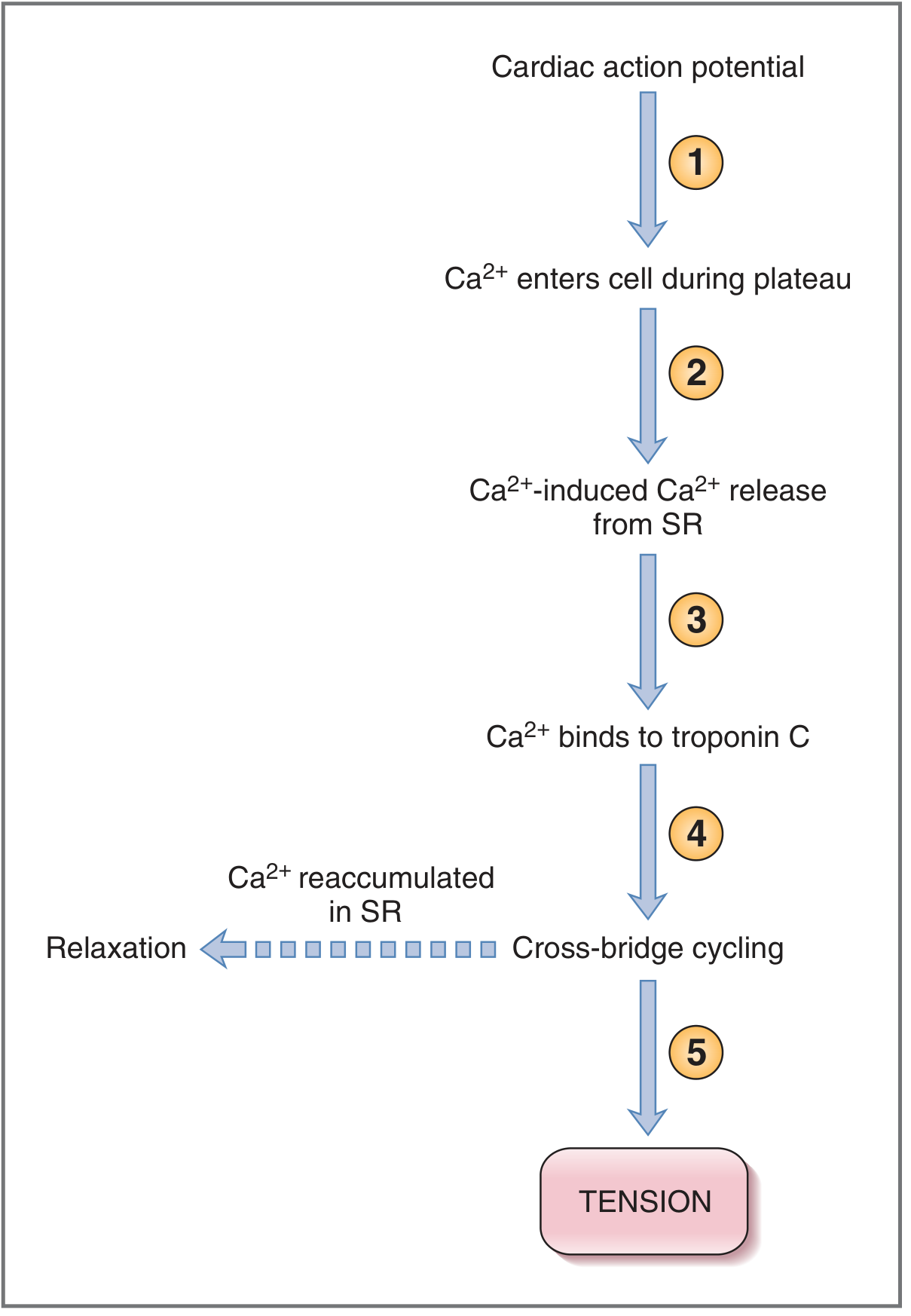
- The cardiac action potential spreads via T tubules to the cell interior.
- During the plateau (phase 2), L-type Ca²⁺ channels (dihydropyridine receptors / Cav1.2) open, and a small amount of Ca²⁺ enters the cell from the ECF. This is "trigger Ca²⁺."
- Trigger Ca²⁺ activates ryanodine receptor 2 (RyR2) channels on the SR, releasing a much larger Ca²⁺ store into the cytoplasm (CICR amplification).
- The rise in [Ca²⁺]i causes Ca²⁺ to bind troponin C, shifting tropomyosin away from the myosin-binding site on actin.
- Actin-myosin cross-bridges form and cycle (powered by ATP hydrolysis), producing tension/shortening via the sliding filament mechanism.
- Tension is proportional to intracellular [Ca²⁺] - this is the key principle governing contractility.
3. Contractility (Inotropy)
| Agent / Mechanism | Effect on Contractility | Mechanism |
|---|---|---|
| Sympathetic stimulation / catecholamines (β₁) | Positive inotropic | ↑cAMP → PKA phosphorylates L-type Ca²⁺ channels (↑Ca²⁺ entry) AND phosphorylates phospholamban (↑SR Ca²⁺ uptake/storage → more Ca²⁺ available next beat; also causes faster relaxation) |
| Digoxin (cardiac glycoside) | Positive inotropic | Inhibits Na⁺/K⁺-ATPase → ↑intracellular Na⁺ → ↓NCX activity → ↑intracellular Ca²⁺ |
| Parasympathetic / ACh (muscarinic) | Negative inotropic (atria) | ↓cAMP → ↓inward Ca²⁺ current; ↑IK-ACh shortens AP plateau |
| Heart failure | Decreased contractility | Depleted SR Ca²⁺ stores, downregulated β₁ receptors |
4. Length-Tension Relationship in Cardiac Muscle
- Optimal sarcomere length (Lmax): ~2.2 µm - maximal actin-myosin overlap, maximum cross-bridge formation, maximum tension.
- Working length at end-diastole: ~1.9 µm (slightly below Lmax), so the heart normally operates on the ascending limb of the length-tension curve.
- Cardiac muscle is much stiffer than skeletal muscle (high resting tension at even modest stretch), so it is "held" on the ascending limb and cannot easily be overstretched beyond Lmax.
- Two additional length-dependent mechanisms unique to cardiac muscle: stretching increases Ca²⁺ sensitivity of troponin C and increases Ca²⁺ release from the SR.
5. Preload and Afterload
- The ventricular wall stretch at the end of diastole, before contraction starts.
- Equivalent to the resting length of the sarcomere just before the beat.
- Clinical surrogates: left ventricular end-diastolic volume (LVEDV), end-diastolic pressure (LVEDP), pulmonary capillary wedge pressure, central venous pressure.
- Governed by the Laplace equation: wall stress = P × R / 2h (where P = pressure, R = radius, h = wall thickness).
- The systolic wall stress on the contracting myocardium after ejection has begun - the load opposing ejection.
- Determined by: aortic pressure, systemic vascular resistance (SVR), aortic compliance, and ventricular wall thickness/geometry.
- Clinical surrogate: systolic blood pressure (adequate unless aortic stenosis is present).
- Aortic impedance (aortic pressure / aortic flow) is the most accurate measure.
- In aortic stenosis or hypertension: afterload ↑ → ventricle compensates by hypertrophy (↑wall thickness, ↓wall stress per Laplace's law).
6. The Frank-Starling Law of the Heart
"The volume of blood ejected by the ventricle in systole depends on the end-diastolic volume (i.e., the venous return)."
- Otto Frank (1895) described the pressure-volume relationship in frog ventricle.
- Ernest Starling (1914) demonstrated in isolated dog hearts that stroke volume is determined by end-diastolic volume.
- Mechanistic basis: as EDV increases → sarcomere length increases → greater actin-myosin overlap + increased Ca²⁺ sensitivity of troponin C → increased force and stroke volume.
- Ensures that in the steady state, cardiac output equals venous return.
- Operates on the ascending limb: at very high EDV, the curve flattens (no further increase) but rarely descends in an intact normal heart (unlike isolated muscle).
- Positive inotropes (e.g., dobutamine, digoxin): shift the curve upward - greater stroke volume for any given EDV.
- Negative inotropes (heart failure): shift the curve downward - reduced stroke volume for any given EDV.
7. Ventricular Pressure-Volume Loop
| Phase | Volume | Pressure | Valves |
|---|---|---|---|
| 1. Diastolic filling (D → A) | Increases (50 → 140 mL) | Low (~5-12 mmHg) | Mitral open, aortic closed |
| 2. Isovolumetric contraction (A → B) | Constant at EDV (~140 mL) | Rises steeply | All valves closed |
| 3. Ventricular ejection (B → C) | Decreases (140 → 70 mL); SV = 70 mL | Rises to ~120 mmHg then falls | Aortic valve open |
| 4. Isovolumetric relaxation (C → D) | Constant at ESV (~70 mL) | Falls to low levels | All valves closed |
- Stroke volume (SV) = width of the loop = EDV - ESV
- Ejection fraction (EF) = SV / EDV × 100 (normal ~55-70%)
- Cardiac output (CO) = SV × heart rate
- Stroke work = area enclosed within the loop = external work done by the ventricle per beat
- Increased preload (↑EDV): loop shifts rightward; wider loop = larger SV (Frank-Starling).
- Increased afterload (↑aortic pressure): loop becomes taller and narrower; ESV rises; SV falls unless compensated.
- Increased contractility: loop shifts to the left; ESV falls dramatically; SV and EF increase.
8. Autonomic Regulation of the Ventricle
| Parameter | Sympathetic (β₁ activation) | Parasympathetic (muscarinic) |
|---|---|---|
| Heart rate (chronotropy) | ↑↑ | ↓↓ (SA node mainly) |
| Contractility (inotropy) | ↑↑ | ↓ (atria only; minimal ventricular effect) |
| Relaxation speed (lusitropy) | ↑ (faster relaxation via phospholamban) | ↓ |
| Conduction velocity (dromotropy) | ↑ | ↓ (AV node slowing) |
9. Ventricular Work and the Fick Principle
10. Law of Laplace Applied to the Ventricle
- The thick LV wall (h ↑) allows it to develop high pressures without excessive wall stress.
- In dilated cardiomyopathy: R ↑ → σ ↑↑ → increased O₂ demand → further ventricular dysfunction.
- In compensatory hypertrophy (aortic stenosis, hypertension): h ↑ → σ normalizes despite high P.
- The ellipsoid shape of the normal LV minimizes wall stress; as the failing LV dilates toward a sphere, wall stress increases substantially.
Summary Table: Key Cardiac Mechanics Concepts
| Concept | Definition | Clinical Correlate |
|---|---|---|
| Preload | Wall stress at end-diastole; sarcomere resting length | ↑ in heart failure with fluid overload |
| Afterload | Wall stress during ejection; opposed by SVR + aortic stiffness | ↑ in hypertension, aortic stenosis |
| Contractility | Intrinsic Ca²⁺-dependent force at given length | ↓ in heart failure; ↑ by catecholamines |
| Frank-Starling law | SV ∝ EDV (venous return) | Ensures cardiac output = venous return |
| Ejection fraction | SV/EDV × 100 | Normal ≥55%; ↓ in systolic HF |
| Stroke work | Area of PV loop | ↑ in volume/pressure overload states |
| Law of Laplace | σ = PR/2h | Basis for compensatory hypertrophy |
control of cardiac pump function physiology
cardiac output venous return curve right atrial pressure Frank-Starling
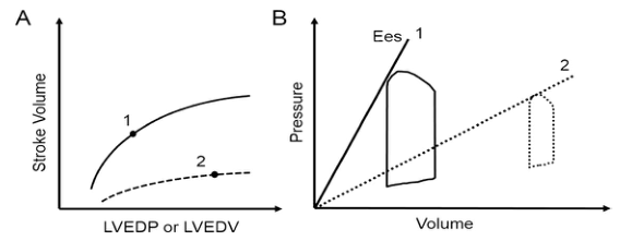
Summary : This figure compares cardiac function under two conditions using two types of plots: (A) the Frank-Starling relationship between stroke volume and left ventricular filling, and (B) pressure-volume loops with end-systolic elastance (Ees) lines. line and schematic plot: # Panel A: Frank-Starling Curve : • Y-axis: Stroke Volume (no units shown). • X-axis: LVEDP or LVEDV (Left Ventricular End-Diastolic Pressure or Volume; no units shown). • Two curves are shown: – Curve 1: Higher, solid line, labeled "1". – Curve 2: Lower, dashed line, labeled "2". • Each curve has a point marked (solid dot) on it. # Panel B: Pressure-Volume Loop and End-Systolic Elastance : • Y-axis: Pressure (no units shown). • X-axis: Volume (no units shown). • Two pressure-volume loops: – Loop 1: Solid line, larger, leftward, labeled "1". – Loop 2: Dashed line, smaller, rightward, labeled "2". • Two Ees (end-systolic elastance) lines: – Ees 1: Steeper, solid line, labeled "1". – Ees 2: Less steep, dashed line, labeled "2". # Design Encodings : • Solid lines for condition 1, dashed lines for condition 2. • Dots mark specific points on the curves in panel A. • Pressure-volume loops are outlined, with loop 2 shown as a dashed outline. # Analysis : • Panel A shows that condition 1 (solid line) has a higher stroke volume for any given LVEDP/LVEDV compared to condition 2 (dashed line), indicating better cardiac function. • Panel B shows that condition 1 has a larger, leftward pressure-volume loop and a steeper Ees line, indicating greater contractility. Condition 2 has a smaller, rightward loop and a less steep Ees line, indicating reduced contractility. • The figure visually contrasts normal/enhanced versus impaired cardiac function using both stroke volume response and pressure-volume relationships.
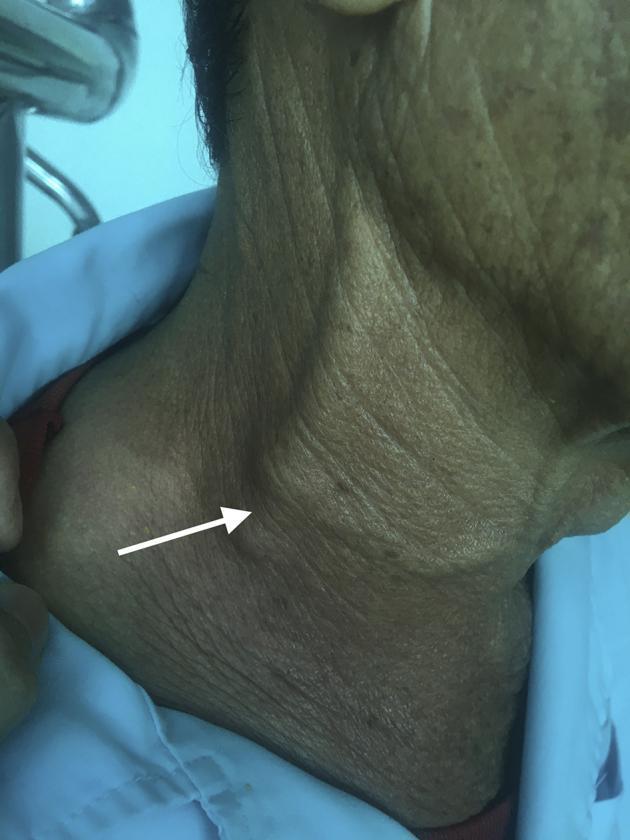
This clinical photograph shows a close-up, lateral view of the right side of an elderly patient's neck, focusing on the lower cervical region. A white arrow points to a distinct, localized swelling located along the anterior border of the right sternocleidomastoid muscle. Visible distension and prominence of the right external jugular vein are observed, suggesting impaired venous return or increased central venous pressure. The overlying skin exhibits age-related changes, including fine wrinkling and solar lentigines. Clinically, these findings represent external manifestations of venous congestion, which may be secondary to superior vena cava syndrome or right atrial compression, leading to internal jugular vein thrombosis. This image serves as an educational example of physical signs associated with thoracic or abdominal masses impacting cardiac inflow.
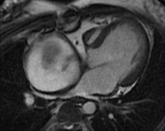
**Imaging Modality:** Cardiac Magnetic Resonance Imaging (MRI), axial steady-state free precession (SSFP) sequence. **Anatomical Region and Landmarks:** Mediastinum and thoracic cavity showing the heart and great vessels in a patient with tricuspid atresia and prior atriopulmonary Fontan palliation. **Observed Pathology:** Severe, aneurysmal dilatation of the right atrium (measuring approximately 7 x 7.5 cm). The massive enlargement of the right atrium causes significant mass effect and posterior displacement of adjacent structures. **Characteristic Visual Features:** - **Atrial Morphometry:** Markedly enlarged, globular right atrium dominant within the thoracic cross-section. - **Vascular Impingement:** The dilated right atrium exerts direct extrinsic compression on the pulmonary venous return pathways. - **Ventricular Morphology:** Single functional ventricle consistent with the surgical history of tricuspid atresia. - **Signal Characteristics:** Blood pool demonstrates typical hyperintense signal on SSFP, highlighting the disproportionate size of the atrial chamber relative to the ventricular mass and the restricted space for pulmonary veins. **Diagnostic Context:** This appearance is characteristic of late complications following an atriopulmonary Fontan connection, where chronic pressure and volume overload lead to progressive giant atrial enlargement and secondary obstructive effects on systemic or pulmonary venous return.
Control of Cardiac Pump Function
1. The Fundamental Principle: Venous Return Drives Cardiac Output
"Venous return is the sum of all local tissue blood flows. Cardiac output regulation is therefore normally determined by local blood flow regulation in all tissues." - Guyton & Hall, p. 252
2. Intrinsic Control Mechanisms
2a. The Frank-Starling Mechanism (Intrinsic Control of Stroke Volume)
- Greater venous return → ↑ right atrial filling → ↑ end-diastolic volume (EDV) → sarcomeres stretched toward optimal overlap → ↑ cross-bridge formation → ↑ contractile force → ↑ stroke volume
- Ensures that in steady state: CO = venous return (otherwise blood would pool)
- Allows the left and right ventricles to stay matched without conscious control
2b. Intrinsic Control of Heart Rate
- Maximum diastolic potential
- Slope of phase 4 depolarization (the "funny current," If)
- Threshold potential
2c. Treppe (Bowditch / Staircase Effect)
3. The Cardiac Function Curve vs. the Vascular Function Curve
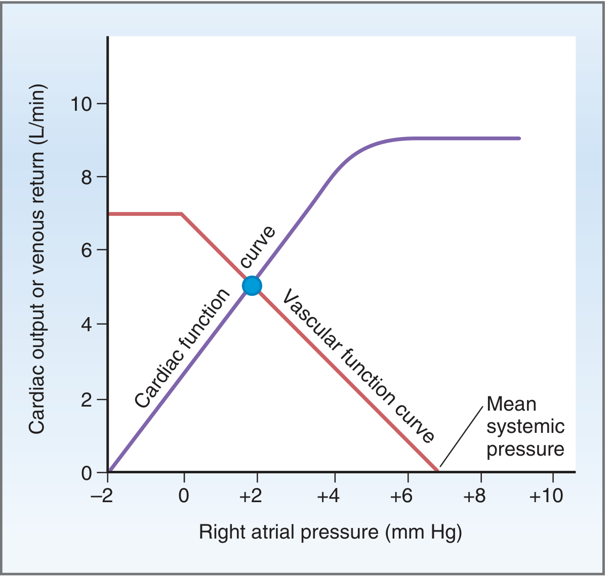
- As RAP ↑ → EDV ↑ → CO ↑ (ascending relationship)
- Plateau at ~9 L/min when RAP ~4 mmHg (heart reaches its pumping limit)
- As RAP ↓ → pressure gradient from systemic veins to right atrium ↑ → venous return ↑ (descending relationship)
- X-intercept = mean systemic filling pressure (~7 mmHg) - the RAP at which venous return = 0
- ↓ TPR (arteriolar dilation) → curve rotates clockwise → ↑ venous return at any RAP
- ↑ TPR (vasoconstriction) → curve rotates counterclockwise → ↓ venous return
4. Extrinsic Control - Autonomic Nervous System
4a. Sympathetic Nervous System
| Effect | Mechanism | Result |
|---|---|---|
| Chronotropy (↑ HR) | ↑ If (funny current) at SA node; steeper phase 4 slope | HR can rise from 70 to >180 bpm |
| Inotropy (↑ contractility) | PKA phosphorylates L-type Ca²⁺ channels → ↑ Ca²⁺ entry; phosphorylates phospholamban → ↑ SERCA activity → ↑ SR Ca²⁺ store | ↑ SV; ↑ EF; cardiac function curve shifts upward |
| Lusitropy (↑ relaxation speed) | Phospholamban phosphorylation speeds Ca²⁺ re-uptake | Faster relaxation allows more filling despite higher HR |
| Dromotropy (↑ AV conduction) | ↑ conduction velocity through AV node | Prevents AV block at high HR |
4b. Parasympathetic Nervous System
| Effect | Mechanism |
|---|---|
| ↓ HR (negative chronotropy) | ↑ IK-ACh → hyperpolarization; ↓ If → shallower phase 4 |
| ↓ AV conduction velocity | Can cause heart block at high vagal tone |
| ↓ Atrial contractility | ↓ cAMP → ↓ inward Ca²⁺ current |
| Minimal ventricular effect | Few parasympathetic terminals reach ventricles |
5. Extrinsic Control - Reflex Mechanisms
5a. High-Pressure Baroreceptors (Carotid Sinus and Aortic Arch)
- Detect stretch in arterial walls (monitor MAP)
- ↑ MAP → baroreceptor firing → NTS → ↑ vagal tone + ↓ sympathetic tone → ↓ HR, ↓ contractility, vasodilation → ↓ CO and ↓ MAP (negative feedback)
- ↓ MAP → opposite response → ↑ HR, ↑ contractility, vasoconstriction → restore MAP
5b. Low-Pressure Baroreceptors (Atrial/Pulmonary Stretch Receptors)
- Atrial distension → Bainbridge reflex: increased sympathetic firing via the vasomotor center → tachycardia (10-15% HR increase from direct stretch; up to 40-60% additional increase via Bainbridge reflex)
- Also triggers renal vasodilation and ANP release → promotes diuresis to reduce volume overload
5c. Chemoreceptor Regulation
- Hypoxia, hypercapnia, acidosis → stimulate chemoreceptors → tachycardia (an important compensatory mechanism)
- Rationale: ↓ CO → ↓ arterial PO₂, ↑ PCO₂ → chemoreceptor activation → ↑ HR → restores CO
6. Extrinsic Control - Humoral / Hormonal Factors
| Agent | Source | Effect on Heart | Mechanism |
|---|---|---|---|
| Catecholamines (epinephrine, norepinephrine) | Adrenal medulla, sympathetic terminals | ↑ HR, ↑ contractility | β₁ receptor → ↑ cAMP |
| Thyroid hormones (T₃, T₄) | Thyroid | ↑ HR, ↑ contractility, ↑ cardiac output; hyperthyroidism → CO 40-80% above normal | ↑ β₁ receptor expression; direct myocardial effects; peripheral vasodilation |
| Glucagon | Pancreas | Positive inotrope and chronotrope | ↑ cAMP (bypasses β₁ receptor) |
| Insulin | Pancreas | Mild positive inotrope | ↑ glucose uptake by myocardium |
| Cortisol | Adrenal cortex | Potentiates catecholamine effects | Permissive upregulation of adrenergic receptors |
| ANP/BNP | Atria/ventricles | Decreased preload (diuresis/vasodilation) | ↑ cGMP → natriuresis |
| Angiotensin II | RAAS | ↑ afterload; direct vasoconstriction | AT₁ receptor |
| Vasopressin (ADH) | Posterior pituitary | ↑ blood volume → ↑ CO | Water retention |
7. Effect of Tissue Metabolism on Cardiac Output
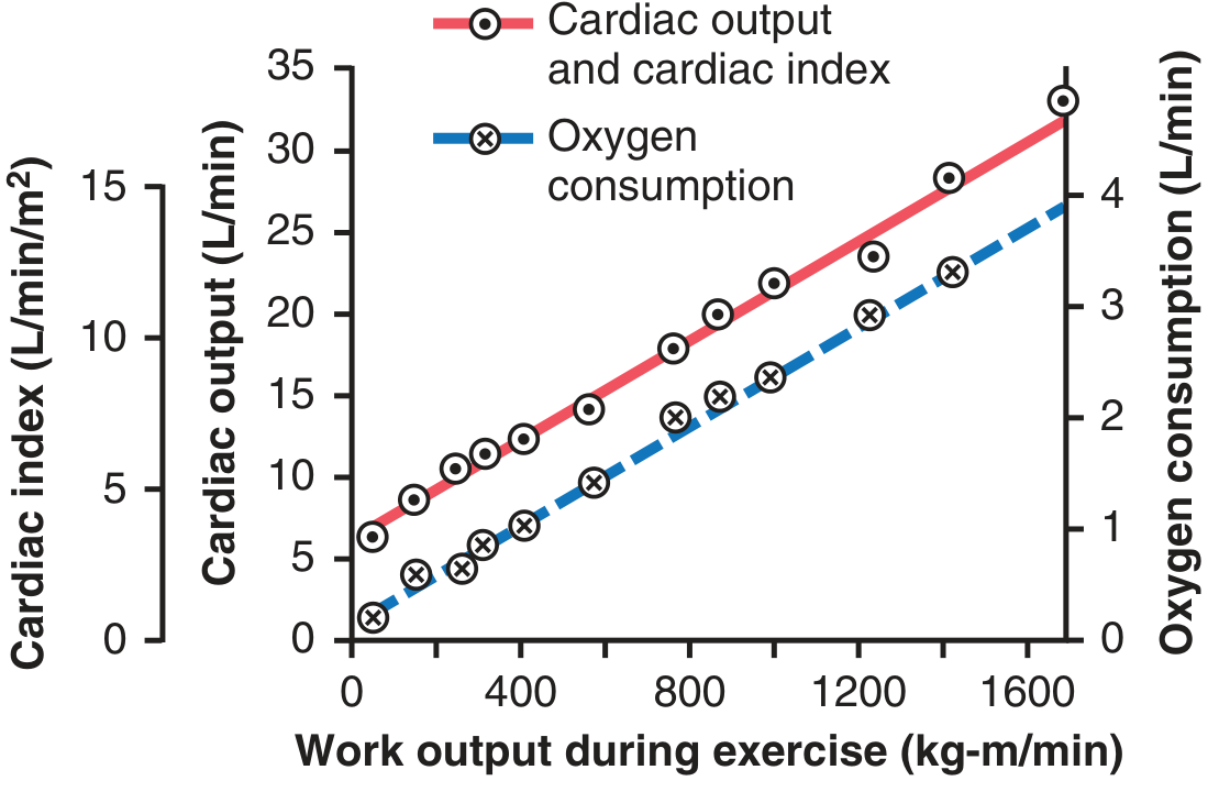
- Active muscle arterioles dilate (metabolic vasodilation: ↑CO₂, ↓O₂, ↑K⁺, adenosine)
- TPR falls → venous return increases
- Frank-Starling raises SV
- Sympathetic activation raises HR and contractility
- Sympathetic venoconstriction raises mean systemic filling pressure
- Net result: CO can increase 4-5× during maximal exercise
8. Role of the Nervous System as an "Enabler"
- With intact nervous system: vasodilation → CO increased ~4-fold with no fall in BP
- Without autonomic control: the same vasodilation caused BP to fall to half-normal and CO increased only 1.6-fold
9. Pathological Alterations in Cardiac Output
- Beriberi (thiamine deficiency) - TPR ↓ to half normal; CO up to 2× normal
- AV fistula - direct arterial-venous shunting → ↓ TPR
- Hyperthyroidism - increased tissue metabolism + peripheral vasodilation; CO 40-80% above normal
- Anemia - reduced blood viscosity + hypoxic vasodilation
- Cardiac factors: MI, valvular disease, myocarditis, tamponade, arrhythmias - heart cannot pump adequate volume
- Venous return factors: Hemorrhage, dehydration, tension pneumothorax, severe peripheral vasoconstriction (cold shock)
10. Summary: Hierarchical Control of CO
CO = HR × SV
      |         |
   Chronotropy  Preload (EDV) via Frank-Starling
      |         Afterload (TPR, aortic pressure)
   Autonomic    Contractility (inotropy)
   Reflexes
   Hormones

Primary controller: VENOUS RETURN (peripheral metabolism)
Modifier:           SYMPATHETIC NERVOUS SYSTEM (HR + inotropy + venoconstriction)
Fine tuner:         PARASYMPATHETIC NERVOUS SYSTEM (HR brake)
Emergency:          HORMONAL (catecholamines, thyroid, RAAS)
| Parameter | Normal Rest | Maximal Exercise |
|---|---|---|
| HR | 60-75 bpm | 180-200 bpm |
| SV | ~70 mL | ~110-130 mL |
| CO | ~5 L/min | 20-30 L/min |
| Cardiac index | ~3 L/min/m² | up to 18 L/min/m² (elite athletes) |
| EF | 55-70% | 70-85% |