Lobes of prostate

Reading File

Finding Sources

Searching Images

lobes zones of prostate anatomy diagram

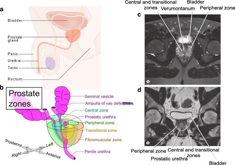
This composite educational graphic illustrates the positional and zonal anatomy of the human prostate gland. Panel (a) is a sagittal schematic showing the prostate’s location inferior to the bladder and anterior to the rectum within the male pelvic cavity. Panel (b) provides a detailed 3D anatomical diagram of the prostate zones as defined by McNeal. It highlights the peripheral zone (posterior/lateral), transitional zone (surrounding the prostatic urethra), central zone (superior/base), and anterior fibromuscular stroma. Associated structures like the seminal vesicles and ampulla of vas deferens are depicted. Panels (c) and (d) present axial and coronal T2-weighted magnetic resonance imaging (MRI) scans, respectively. These diagnostic images correlate the schematic zones to clinical findings, identifying the hyperintense peripheral zone and relatively hypointense central/transitional zones. Key landmarks labeled include the bladder, verumontanum, and prostatic urethra. This resource is designed for medical education to aid in the radiological and clinical localization of prostate pathologies such as BPH and adenocarcinoma.

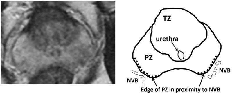
An educational figure combining an axial MRI image (left) and a corresponding anatomical schematic (right) of the prostate gland. The content illustrates the zonal anatomy of the prostate and its spatial relationship to adjacent structures. The diagram identifies the transition zone (TZ) as the central region, containing the urethra. Surrounding the posterior and lateral aspects of the TZ is the peripheral zone (PZ). Notably, the schematic highlights the 'edge of PZ in proximity to NVB' using a dotted line, where the peripheral zone borders the bilateral neurovascular bundles (NVB). This clinical illustration is designed to teach the anatomical landmarks relevant to focal therapies, such as High-Intensity Focused Ultrasound (HIFU), where the distance between the treatment area in the peripheral zone and the neurovascular bundle is a critical factor for preserving post-operative erectile function. The modality demonstrated is T2-weighted magnetic resonance imaging, which provides the soft-tissue contrast necessary to distinguish between prostatic zones.

A multi-panel medical graphic illustrating the diagnostic workflow for prostate cancer staging and image fusion. On the left, axial views of the pelvis demonstrate two imaging modalities: a [68Ga]Ga-PSMA-11 PET scan showing metabolic activity (hotspot) in the prostate gland with a green contour, and an MRI-derived Apparent Diffusion Coefficient (ADC) map showing tissue density with a red contour. The central element is an anatomical schematic diagram of the prostate base, divided into labeled zones: anterior fibromuscular stroma (AFS), anterior/posterior transition zones (TZa/p), anterior/posterior peripheral zones (PZa/p), and the central zone (CZ). A red circle on the schematic identifies a lesion in the right posterior peripheral zone (PZp), corresponding to histological findings of acinar adenocarcinoma (ISUP 3). The right panel shows the fusion of PET and ADC images using MIM maestro software, overlaying metabolic and structural data to refine tumor localization. This image serves as an educational resource for radiomics, multi-modal image registration, and prostate zonal anatomy in the context of oncological pathology.

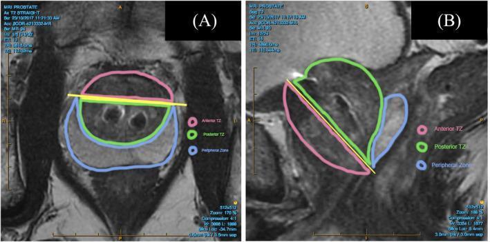
Two T2-weighted magnetic resonance imaging (MRI) scans of the human prostate gland in axial (A) and sagittal (B) planes, annotated to delineate zonal anatomy. The images highlight three distinct regions: the Anterior Transition Zone (outlined in pink), the Posterior Transition Zone (outlined in green), and the Peripheral Zone (outlined in blue). In the axial view, a yellow horizontal line marks the confluence of the peripheral and transition zones. In the sagittal view, a yellow line extends from the anterior urethra to the distal extension of the peripheral zone, acting as a boundary between the anterior and posterior transition zones. The peripheral zone is characterized by higher signal intensity (brighter appearance) compared to the transition zones. These images are used to demonstrate prostate anatomy and the spatial relationship between zones, which is critical for identifying pathology such as benign prostatic hyperplasia (BPH) and prostate cancer, or assessing metal artifacts from urethral implants.

Finding Sources

Reading File

Loading Image

Finding Sources

Reading File

Loading Image

Here is a thorough breakdown of the Lobes of the Prostate:

Lobes of the Prostate

The prostate can be described using two complementary frameworks: the classical lobe system (used clinically and at cystoscopy) and the zone system (McNeal, used in pathology and radiology).

1. Classical Lobe Classification (5 Lobes)

As described in Smith and Tanagho's General Urology (19th ed.):

"The lobe classification is often used in cystourethroscopic examinations and consists of five lobes: anterior, posterior, median, right lateral, and left lateral."

Lobe	Location	Clinical Relevance
Anterior lobe	In front of the urethra	Largely fibromuscular; rarely involved in pathology
Posterior lobe	Behind the urethra, palpable on DRE	Prone to cancerous degeneration (most prostate cancers)
Median (middle) lobe	Between urethra and ejaculatory ducts	Prone to BPH; can protrude into the bladder neck causing obstruction
Right lateral lobe	Right side of urethra	Together with left lateral lobe = bulk of the gland; main site of BPH
Left lateral lobe	Left side of urethra	Same as above

A central sulcus divides the two lateral lobes, palpable on digital rectal examination. The median lobe may become hyperplastic and extend into the bladder neck with age.

Smith and Tanagho's General Urology, 19th Ed., p. 22
Campbell Walsh Wein Urology, p. 1818

2. McNeal Zone Classification (Modern, Pathological)

McNeal (1981/1988) re-described the prostate into 4 zones, which correlate better with disease:

McNeal zones of the prostate - sagittal diagram showing peripheral, central, transition zones and anterior fibromuscular stroma

Prostate zones 3D diagram and MRI correlation

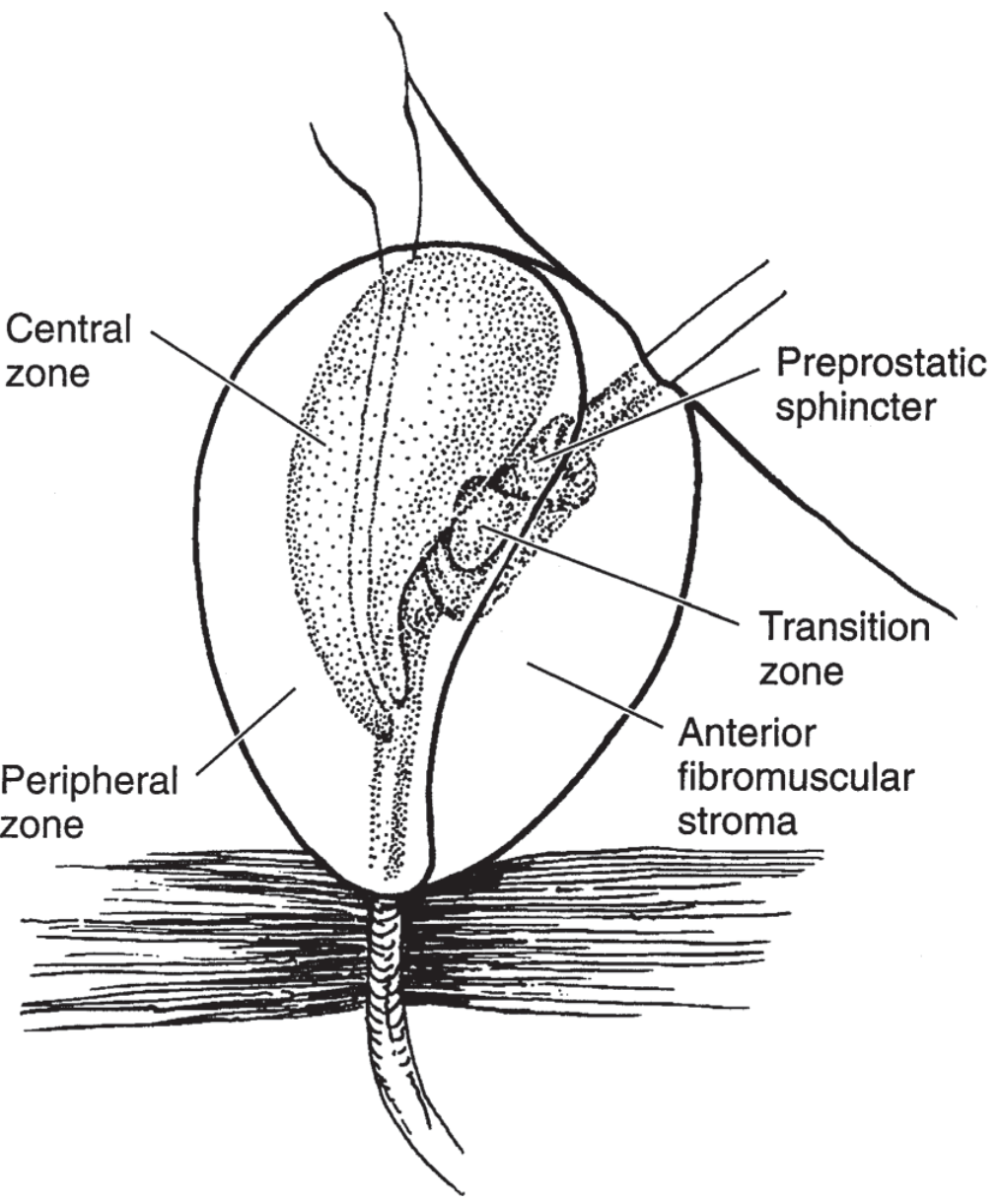
Zone	Size (% glandular tissue)	Location	Disease Association
Peripheral zone (PZ)	~70%	Posterior and lateral aspects	70% of prostate cancers originate here; palpable on DRE
Central zone (CZ)	~25%	Surrounds ejaculatory ducts; projects under bladder base	Wolffian duct origin; rarely affected by disease
Transition zone (TZ)	~5% (in youth)	Surrounds the urethra proximal to ejaculatory ducts	Almost exclusively the site of BPH
Anterior fibromuscular stroma (AFS)	Non-glandular	From bladder neck to striated sphincter; up to 1/3 of prostate mass	No glandular tissue; composed of collagen, smooth/striated muscle, elastin

Campbell Walsh Wein Urology, p. 1818
Smith and Tanagho's General Urology, p. 22

Key Clinical Correlations

Condition	Zone/Lobe Involved
BPH (benign prostatic hyperplasia)	Transition zone + median lobe (periurethral glands)
Prostate cancer	Peripheral zone (70%), transition zone (20%), central zone (10%)
DRE palpation	Posterior lobe / peripheral zone
Prostatic urethral lift (PUL)	Lateral lobes only; not appropriate for median lobe enlargement

Gross Anatomy Note

Weight: ~18-20 g (normal)
Dimensions: 3 cm length, 4 cm width, 2 cm depth
The prostatic urethra (~2.5 cm) traverses the gland
The verumontanum on the urethral floor marks where ejaculatory ducts open
No true capsule exists at the apex or at the bladder base junction
Campbell Walsh Wein Urology, p. 1817-1818

Can you create a chart of prostate lobe

Asking for Preferences

Reading File

Running Command

mkdir -p /tmp/workspace/prostate-chart && ls /tmp/workspace/prostate-chart/

Writing File

~/prostate-chart/generate_chart.py

from reportlab.lib.pagesizes import A4
from reportlab.lib import colors
from reportlab.lib.styles import getSampleStyleSheet, ParagraphStyle
from reportlab.lib.units import cm
from reportlab.platypus import (
    SimpleDocTemplate, Table, TableStyle, Paragraph,
    Spacer, HRFlowable
)
from reportlab.lib.enums import TA_CENTER, TA_LEFT

OUTPUT = "/tmp/workspace/prostate-chart/Prostate_Lobes_Chart.pdf"

doc = SimpleDocTemplate(
    OUTPUT,
    pagesize=A4,
    leftMargin=1.5*cm,
    rightMargin=1.5*cm,
    topMargin=1.5*cm,
    bottomMargin=1.5*cm,
)

styles = getSampleStyleSheet()

# Custom styles
title_style = ParagraphStyle(
    "Title",
    parent=styles["Title"],
    fontSize=20,
    textColor=colors.HexColor("#1a3a5c"),
    spaceAfter=4,
    alignment=TA_CENTER,
    fontName="Helvetica-Bold",
)
subtitle_style = ParagraphStyle(
    "Subtitle",
    parent=styles["Normal"],
    fontSize=11,
    textColor=colors.HexColor("#4a6fa5"),
    spaceAfter=10,
    alignment=TA_CENTER,
    fontName="Helvetica-Oblique",
)
section_style = ParagraphStyle(
    "Section",
    parent=styles["Normal"],
    fontSize=13,
    textColor=colors.white,
    fontName="Helvetica-Bold",
    alignment=TA_CENTER,
)
cell_style = ParagraphStyle(
    "Cell",
    parent=styles["Normal"],
    fontSize=9,
    leading=12,
    fontName="Helvetica",
    alignment=TA_LEFT,
)
cell_bold = ParagraphStyle(
    "CellBold",
    parent=styles["Normal"],
    fontSize=9,
    leading=12,
    fontName="Helvetica-Bold",
    alignment=TA_LEFT,
)
footnote_style = ParagraphStyle(
    "Footnote",
    parent=styles["Normal"],
    fontSize=8,
    textColor=colors.HexColor("#666666"),
    alignment=TA_CENTER,
    fontName="Helvetica-Oblique",
)

# ---------------------------------------------------------------
# SECTION HEADER helper
# ---------------------------------------------------------------
def section_header(text, bg_color):
    return Table(
        [[Paragraph(text, section_style)]],
        colWidths=[17.7*cm],
        rowHeights=[0.65*cm],
        style=TableStyle([
            ("BACKGROUND", (0, 0), (-1, -1), bg_color),
            ("ROUNDEDCORNERS", [4, 4, 4, 4]),
            ("VALIGN", (0, 0), (-1, -1), "MIDDLE"),
        ]),
    )

# ---------------------------------------------------------------
# PART 1 – Classical Five-Lobe Classification
# ---------------------------------------------------------------
BLUE_DARK  = colors.HexColor("#1a3a5c")
BLUE_MED   = colors.HexColor("#2e6da4")
BLUE_LIGHT = colors.HexColor("#d6e8f7")
BLUE_ALT   = colors.HexColor("#eaf3fb")
GREEN_DARK = colors.HexColor("#1a5c3a")
GREEN_MED  = colors.HexColor("#2e9b5e")
GREEN_LIGHT= colors.HexColor("#d6f7e8")
GREEN_ALT  = colors.HexColor("#eafbf3")
RED_HIGH   = colors.HexColor("#c0392b")
ORANGE     = colors.HexColor("#e67e22")
GRAY_LIGHT = colors.HexColor("#f5f5f5")

def p(text, style=cell_style):
    return Paragraph(text, style)

def pb(text):
    return Paragraph(text, cell_bold)

# Column headers for lobe table
lobe_headers = [
    pb("Lobe"),
    pb("Position"),
    pb("Histology"),
    pb("Clinical Relevance"),
    pb("Pathology"),
]

lobe_data = [
    [
        p("<b>Anterior\nLobe</b>"),
        p("Anterior to\nthe urethra"),
        p("Largely\nfibromuscular;\nminimal glands"),
        p("Not palpable\non DRE"),
        p("Rarely involved\nin disease"),
    ],
    [
        p("<b>Posterior\nLobe</b>"),
        p("Posterior to\nthe urethra;\npalpable on DRE"),
        p("True glandular\ntissue"),
        p("Palpated directly\nvia digital rectal\nexamination"),
        p("<font color='#c0392b'><b>Primary site of\nprostate cancer\n(carcinoma)</b></font>"),
    ],
    [
        p("<b>Median\n(Middle)\nLobe</b>"),
        p("Between urethra\nand ejaculatory\nducts"),
        p("Glandular;\nperiurethral\nglands"),
        p("Can protrude\ninto bladder neck\n(intravesical IPP)"),
        p("<font color='#e67e22'><b>Main site of BPH;\nobstructs urine\nflow</b></font>"),
    ],
    [
        p("<b>Right\nLateral\nLobe</b>"),
        p("Right side\nof urethra"),
        p("Predominantly\nglandular tissue"),
        p("Palpable on DRE;\nbulk of prostate\nmass"),
        p("BPH; lateral lobe\nhypertrophy causing\nLUTS"),
    ],
    [
        p("<b>Left\nLateral\nLobe</b>"),
        p("Left side\nof urethra"),
        p("Predominantly\nglandular tissue"),
        p("Palpable on DRE;\nbulk of prostate\nmass"),
        p("BPH; lateral lobe\nhypertrophy causing\nLUTS"),
    ],
]

col_w = [2.8*cm, 3.3*cm, 3.3*cm, 3.7*cm, 4.6*cm]

lobe_table_data = [lobe_headers] + lobe_data
lobe_table = Table(lobe_table_data, colWidths=col_w, repeatRows=1)
lobe_table.setStyle(TableStyle([
    # Header row
    ("BACKGROUND",   (0, 0), (-1, 0),  BLUE_DARK),
    ("TEXTCOLOR",    (0, 0), (-1, 0),  colors.white),
    ("FONTNAME",     (0, 0), (-1, 0),  "Helvetica-Bold"),
    ("FONTSIZE",     (0, 0), (-1, 0),  9),
    ("ALIGN",        (0, 0), (-1, 0),  "CENTER"),
    ("VALIGN",       (0, 0), (-1, -1), "MIDDLE"),
    # Alternating rows
    ("BACKGROUND",   (0, 1), (-1, 1),  BLUE_LIGHT),
    ("BACKGROUND",   (0, 2), (-1, 2),  BLUE_ALT),
    ("BACKGROUND",   (0, 3), (-1, 3),  BLUE_LIGHT),
    ("BACKGROUND",   (0, 4), (-1, 4),  BLUE_ALT),
    ("BACKGROUND",   (0, 5), (-1, 5),  BLUE_LIGHT),
    # Grid
    ("GRID",         (0, 0), (-1, -1), 0.4, colors.HexColor("#a0b8cc")),
    ("ROWBACKGROUND",(0, 0), (-1, 0),  BLUE_DARK),
    ("TOPPADDING",   (0, 0), (-1, -1), 5),
    ("BOTTOMPADDING",(0, 0), (-1, -1), 5),
    ("LEFTPADDING",  (0, 0), (-1, -1), 5),
    ("RIGHTPADDING", (0, 0), (-1, -1), 5),
]))

# ---------------------------------------------------------------
# PART 2 – McNeal Zone Classification
# ---------------------------------------------------------------
zone_headers = [
    pb("Zone"),
    pb("% Glandular\nTissue"),
    pb("Location"),
    pb("Ducts / Drainage"),
    pb("Disease Association"),
]

zone_data = [
    [
        p("<b>Peripheral\nZone (PZ)</b>"),
        p("<b>~70%</b>\n(largest zone)"),
        p("Posterior and lateral\naspects; apical region"),
        p("Drain into prostatic\nsinus along entire\npostsphincteric urethra"),
        p("<font color='#c0392b'><b>70% of prostate\ncancers originate\nhere</b></font>"),
    ],
    [
        p("<b>Central\nZone (CZ)</b>"),
        p("<b>~25%</b>"),
        p("Surrounds ejaculatory\nducts; projects under\nbladder base"),
        p("Ejaculatory duct\norifices at\nverumontanum"),
        p("Wolffian duct origin;\nrarely affected\nby disease"),
    ],
    [
        p("<b>Transition\nZone (TZ)</b>"),
        p("<b>~5%</b>\n(youth; enlarges\nwith age)"),
        p("Surrounds urethra\nproximal to\nejaculatory ducts"),
        p("Ducts begin at\npreprostatic/prostatic\nurethra angle"),
        p("<font color='#e67e22'><b>Almost exclusively\nthe site of BPH</b></font>"),
    ],
    [
        p("<b>Anterior\nFibromuscular\nStroma (AFS)</b>"),
        p("<b>Non-glandular</b>\n(up to 1/3 of\nmass)"),
        p("Anterior surface;\nbladder neck to\nstriated sphincter"),
        p("No glandular\nelements"),
        p("Composed of\ncollagen, smooth\n& striated muscle,\nelastin"),
    ],
]

zone_col_w = [3.2*cm, 3.0*cm, 3.7*cm, 3.8*cm, 4.0*cm]

zone_table_data = [zone_headers] + zone_data
zone_table = Table(zone_table_data, colWidths=zone_col_w, repeatRows=1)
zone_table.setStyle(TableStyle([
    ("BACKGROUND",   (0, 0), (-1, 0),  GREEN_DARK),
    ("TEXTCOLOR",    (0, 0), (-1, 0),  colors.white),
    ("FONTNAME",     (0, 0), (-1, 0),  "Helvetica-Bold"),
    ("FONTSIZE",     (0, 0), (-1, 0),  9),
    ("ALIGN",        (0, 0), (-1, 0),  "CENTER"),
    ("VALIGN",       (0, 0), (-1, -1), "MIDDLE"),
    ("BACKGROUND",   (0, 1), (-1, 1),  GREEN_LIGHT),
    ("BACKGROUND",   (0, 2), (-1, 2),  GREEN_ALT),
    ("BACKGROUND",   (0, 3), (-1, 3),  GREEN_LIGHT),
    ("BACKGROUND",   (0, 4), (-1, 4),  GREEN_ALT),
    ("GRID",         (0, 0), (-1, -1), 0.4, colors.HexColor("#7dbf99")),
    ("TOPPADDING",   (0, 0), (-1, -1), 5),
    ("BOTTOMPADDING",(0, 0), (-1, -1), 5),
    ("LEFTPADDING",  (0, 0), (-1, -1), 5),
    ("RIGHTPADDING", (0, 0), (-1, -1), 5),
]))

# ---------------------------------------------------------------
# PART 3 – Quick Clinical Correlation summary table
# ---------------------------------------------------------------
corr_headers = [pb("Condition"), pb("Lobe / Zone Involved"), pb("Key Feature")]
corr_data = [
    [p("Benign Prostatic Hyperplasia (BPH)"),
     p("Transition Zone + Median Lobe"),
     p("Periurethral gland proliferation → urinary obstruction")],
    [p("Prostate Cancer (most common)"),
     p("Peripheral Zone (70%)"),
     p("Palpable on DRE; detected by PSA + biopsy")],
    [p("Prostate Cancer (less common)"),
     p("Transition Zone (20%), Central Zone (10%)"),
     p("Often found incidentally on TURP chips")],
    [p("Digital Rectal Examination (DRE)"),
     p("Posterior Lobe / Peripheral Zone"),
     p("Only palpable part; assesses nodularity or induration")],
    [p("Intravesical Protrusion"),
     p("Median (Middle) Lobe"),
     p("IPP = intravesical prostatic protrusion; causes AUR")],
    [p("Prostatic Urethral Lift (PUL)"),
     p("Lateral Lobes only"),
     p("NOT appropriate if median lobe is enlarged")],
]

corr_col_w = [4.5*cm, 5.5*cm, 7.7*cm]
corr_table_data = [corr_headers] + corr_data
corr_table = Table(corr_table_data, colWidths=corr_col_w, repeatRows=1)
corr_table.setStyle(TableStyle([
    ("BACKGROUND",   (0, 0), (-1, 0),  colors.HexColor("#4a4a6a")),
    ("TEXTCOLOR",    (0, 0), (-1, 0),  colors.white),
    ("FONTNAME",     (0, 0), (-1, 0),  "Helvetica-Bold"),
    ("FONTSIZE",     (0, 0), (-1, 0),  9),
    ("ALIGN",        (0, 0), (-1, 0),  "CENTER"),
    ("VALIGN",       (0, 0), (-1, -1), "MIDDLE"),
    ("ROWBACKGROUNDS",(0, 1), (-1, -1), [colors.HexColor("#eeeef5"), colors.white]),
    ("GRID",         (0, 0), (-1, -1), 0.4, colors.HexColor("#9999bb")),
    ("TOPPADDING",   (0, 0), (-1, -1), 5),
    ("BOTTOMPADDING",(0, 0), (-1, -1), 5),
    ("LEFTPADDING",  (0, 0), (-1, -1), 5),
    ("RIGHTPADDING", (0, 0), (-1, -1), 5),
]))

# ---------------------------------------------------------------
# BUILD STORY
# ---------------------------------------------------------------
story = []

story.append(Paragraph("LOBES OF THE PROSTATE", title_style))
story.append(Paragraph("Comprehensive Reference Chart — Lobe & Zone Classification", subtitle_style))
story.append(HRFlowable(width="100%", thickness=2, color=BLUE_DARK, spaceAfter=8))

# Part 1
story.append(section_header("PART 1: Classical Five-Lobe Classification  (Clinical / Cystoscopic)", BLUE_MED))
story.append(Spacer(1, 0.2*cm))
story.append(lobe_table)
story.append(Spacer(1, 0.3*cm))

# Part 2
story.append(section_header("PART 2: McNeal Zone Classification  (Pathological / Radiological)", GREEN_MED))
story.append(Spacer(1, 0.2*cm))
story.append(zone_table)
story.append(Spacer(1, 0.3*cm))

# Part 3
story.append(section_header("PART 3: Clinical Correlations at a Glance", colors.HexColor("#4a4a6a")))
story.append(Spacer(1, 0.2*cm))
story.append(corr_table)
story.append(Spacer(1, 0.4*cm))

story.append(HRFlowable(width="100%", thickness=1, color=colors.HexColor("#aaaaaa"), spaceAfter=4))
story.append(Paragraph(
    "Sources: Smith & Tanagho's General Urology 19th Ed. | Campbell Walsh Wein Urology | McNeal JE, Prostate 1981;2(1):35–49",
    footnote_style
))

doc.build(story)
print("PDF created:", OUTPUT)

Running Command

python /tmp/workspace/prostate-chart/generate_chart.py

Your PDF chart is ready. It contains three structured tables on a single A4 page:

Part 1 - Classical Five-Lobe Classification (Anterior, Posterior, Median, Right & Left Lateral) with position, histology, clinical relevance, and pathology
Part 2 - McNeal Zone Classification (Peripheral, Central, Transition, Anterior Fibromuscular Stroma) with percentages, locations, and disease associations
Part 3 - Clinical Correlations at a glance (BPH, prostate cancer, DRE, IPP, PUL)

Prostate Lobes Chart

PDF Document · PDF

Diagram of the lobe of prostate

Generating Image

Medical anatomy diagram of the lobes of the prostate gland, clean educational illustration showing two views: 1) A cross-sectional (axial/transverse) view from above labeling the five classical lobes: Anterior Lobe (front), Posterior Lobe (back), Median/Middle Lobe (center between urethra and ejaculatory ducts), Right Lateral Lobe, and Left Lateral Lobe, with the prostatic urethra in the center; 2) A sagittal side-view showing the McNeal zones: Peripheral Zone (posterior/lateral, largest, ~70%), Central Zone (surrounds ejaculatory ducts, ~25%), Transition Zone (surrounds urethra, ~5%), and Anterior Fibromuscular Stroma (front). Each zone and lobe labeled with clear arrows, different colors for each region, bladder above and urethra below shown for anatomical context. White background, professional medical textbook style, no extra text outside labels.

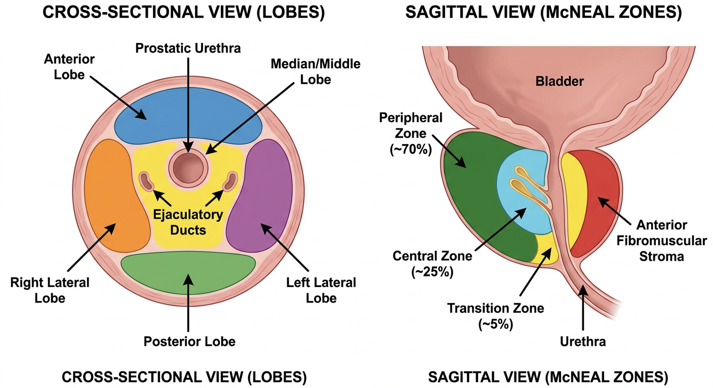
The diagram shows both classification systems side by side:

Classical 5-Lobe System (cross-section view)

Anterior lobe - in front of the urethra; largely fibromuscular
Posterior lobe - behind the urethra; main site of prostate cancer
Median (middle) lobe - between urethra and ejaculatory ducts; main site of BPH
Right & Left lateral lobes - bulk of the gland; also involved in BPH

McNeal Zones (sagittal view)

Peripheral zone (~70%) - posterior/lateral; 70% of cancers here
Central zone (~25%) - around ejaculatory ducts; rarely diseased
Transition zone (~5%) - around urethra; exclusively site of BPH
Anterior fibromuscular stroma - non-glandular front portion

This is a shared conversation. Sign in to Orris to start your own chat.