summarization of data, measures of central tendency, averages

Reading File

Searching the Web

measures of central tendency averages summarization of data statistics

Finding Sources

Reading File

Loading Image

I now have all the material needed for a thorough, well-sourced answer. Here is the full response:

Summarization of Data, Measures of Central Tendency & Averages

What Is Data Summarization?

Descriptive statistics condense large sets of observations into a few representative numbers. In any study or dataset, continuous variables (age, weight, lab values) are typically described with two complementary statistics:

A measure of central tendency - a single value representing where data clusters
A measure of spread - indicating variability around that center (standard deviation, range, IQR)

This summary is the foundation of presenting baseline characteristics in research and clinical studies. - Rockwood and Green's Fractures in Adults, 10th ed., p. [block 3]

The Three Core Measures of Central Tendency

1. Mean (Arithmetic Mean) - Parametric

The mean is the most widely recognized measure of central tendency:

$$\bar{x} = \frac{x_1 + x_2 + \cdots + x_n}{n} = \frac{\sum_{i=1}^n x_i}{n}$$

Calculated from a defined formula - therefore called a parametric method
Sensitive to outliers and extreme values
Best used when data are normally (Gaussian) distributed
The preferred summary statistic for normally distributed continuous data

Example: Patient ages 45, 50, 55, 60, 65 → Mean = 275/5 = 55 years

2. Median - Nonparametric

The median divides all data points exactly in half - one half above, one half below. It is also called the 50th percentile.

Not derived from a formula - taken from a direct count of data points - therefore called a nonparametric method
Resistant to outliers and extreme values
Preferred when data are skewed or non-normally distributed
Appropriate for ordinal variables (e.g., pain scales 0-5)

Example: Ages 45, 50, 55, 60, 90 → Median = 55 years (mean would be 60, pulled up by outlier 90)

3. Mode

The mode is the most frequently occurring value in a dataset.

Not very useful for describing or comparing most datasets
Has a role when a dataset consists of two or more subpopulations (called a bimodal distribution)
Skewed data does NOT affect the mode
Henry's Clinical Diagnosis and Management by Laboratory Methods
Quick Compendium of Clinical Pathology, 5th ed.

The Geometric Mean

The geometric mean minimizes the influence of extreme values and is calculated as the nth root of the product of all n values:

$$\text{Geometric Mean} = \sqrt[n]{x_1 \times x_2 \times \cdots \times x_n}$$

A mathematically equivalent and more convenient formula:

$$\log(\text{Geometric Mean}) = \frac{\sum_{i=1}^n \log x_i}{n}$$

(Take the antilog of the result to get the geometric mean.)

When to use it: When data are heavily skewed toward lower values with some high outliers. For example, the dataset 3, 3, 4, 4, 5, 5, 5, 6, 6, 8, 9, 10, 15, 21 has:

Arithmetic mean = 7.2
Geometric mean = 6.09 (better reflects the preponderance of low values)

The geometric mean is also appropriate for ratios, growth rates, and logarithmically distributed data (e.g., antibody titers, infection rates).

Henry's Clinical Diagnosis and Management by Laboratory Methods

Relationship Between Mean, Median & Mode in Different Distributions

Distribution	Relationship	Best Measure
Symmetric (normal/Gaussian)	Mean = Median = Mode	Mean
Positively skewed (right tail)	Mean > Median > Mode	Median
Negatively skewed (left tail)	Mean < Median < Mode	Median
Bimodal	Two peaks	Mode (or report both peaks)

In a positively skewed dataset, the mean is pulled toward the high-value tail, making it unrepresentative. The median is more stable. - Quick Compendium of Clinical Pathology, 5th ed.

The Normal (Gaussian) Distribution

The Gaussian distribution is symmetric and bell-shaped, centered on the mean. In a perfect Gaussian distribution, mean = median = mode.

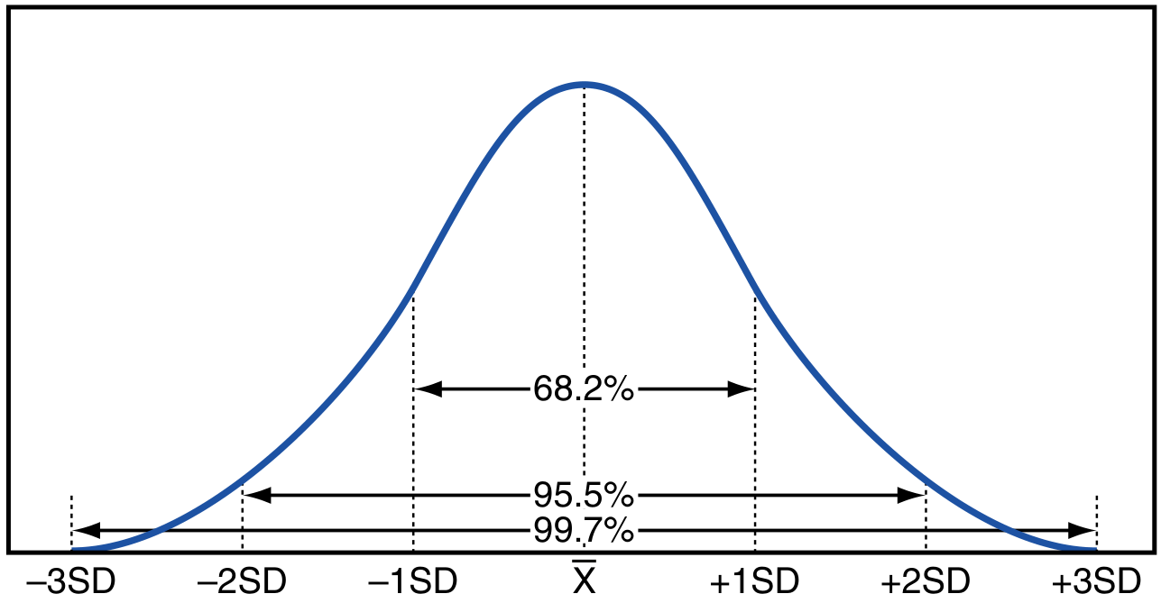
Idealized Gaussian (normal) distribution showing areas under the curve at ±1, ±2, and ±3 standard deviations

Figure: Areas under the normal curve - Henry's Clinical Diagnosis

Range	% of Data Included
Mean ± 1 SD	68.2%
Mean ± 2 SD	95.5%
Mean ± 3 SD	99.7%

Measures of Spread (Alongside Central Tendency)

Central tendency alone is incomplete. Spread must always be reported:

Measure	Used With	Notes
Standard Deviation (SD)	Mean (normal data)	SD = √[Σ(x - mean)²/(n-1)]
Range	Median (skewed data)	Lowest to highest value
Interquartile Range (IQR)	Median (skewed data)	Middle 50% of values (excludes top and bottom quartiles)

Rockwood and Green's Fractures in Adults

Parametric vs. Nonparametric Summary

Feature	Parametric (Mean)	Nonparametric (Median)
Assumes distribution?	Yes (normal)	No
Sensitive to outliers?	Yes	No
Enables further statistical tests?	Many (t-test, ANOVA)	Fewer (Mann-Whitney, etc.)
Best data type	Continuous, normally distributed	Skewed, ordinal, or non-normal

Quick Selection Guide

Normally distributed continuous data (e.g., height, weight, lab values in healthy population) → Mean ± SD
Skewed continuous data (e.g., income, hospital length of stay, troponin levels) → Median [IQR]
Ordinal data (e.g., pain scale, functional scores) → Median
Categorical/nominal data → Frequency and proportion (%)
Ratio/growth rate data → Geometric mean

Sources: Henry's Clinical Diagnosis and Management by Laboratory Methods; Quick Compendium of Clinical Pathology, 5th ed.; Rockwood and Green's Fractures in Adults, 10th ed. 2025; Australian Bureau of Statistics - Central Tendency

what is measure of central tendency and average we dont have to calculate

Measures of Central Tendency & Averages (Conceptual Only)

What is a Measure of Central Tendency?

A measure of central tendency is a single value that represents or summarizes an entire dataset by indicating where the data tends to cluster or concentrate - the "center" of the data.

Think of it as the answer to: "What is the typical or most representative value in this data?"

The Three Main Measures

1. 📊 MEAN (Arithmetic Average)

"The fair share value"

The mean is what you get if all values were equally distributed among everyone.

It is the most commonly used average
Uses ALL values in the data
Also called the arithmetic mean
It is a parametric measure (based on a formula)

Weakness: Gets pulled by extreme values (outliers)

Example concept: If 5 students scored differently on a test, the mean is what each student would have scored if everyone got the same marks.

2. 📍 MEDIAN

"The middle value"

The median is the middle value when data is arranged in order. Exactly half the values fall above it and half below.

Also called the 50th percentile
It is a non-parametric measure (based on counting, not a formula)
NOT affected by outliers - this is its biggest advantage

When to use: When data is skewed or has extreme values (e.g., income data, hospital stay lengths)

Example concept: In a street where most houses cost ₹50 lakh but one costs ₹5 crore, the median house price gives a more honest picture than the mean.

3. 🔢 MODE

"The most popular value"

The mode is the value that appears most frequently in the dataset.

A dataset can have no mode, one mode (unimodal), or two modes (bimodal)
Most useful for categorical data (e.g., most common blood group, most popular shoe size)
Not affected by skewness

Example concept: The most commonly sold dress size in a store is the mode.

Other Types of Averages

Average	What It Represents	Best Used For
Arithmetic Mean	Equal distribution of total	Symmetric, normal data
Median	Middle value	Skewed data, outliers present
Mode	Most frequent value	Categorical data, bimodal data
Geometric Mean	Accounts for extreme high values	Ratios, growth rates, antibody titers
Harmonic Mean	Based on reciprocals	Speed, rates

Simple Analogy for All Three

Imagine 5 friends have these amounts of money: ₹10, ₹20, ₹20, ₹30, ₹100

Measure	Value	Meaning
Mean	₹36	Total shared equally - pulled up by ₹100
Median	₹20	Middle value - more realistic
Mode	₹20	Most common amount

The ₹100 outlier dragged the mean up, but median and mode remained honest.

When to Use Which?

Is the data normally distributed (bell-shaped)?
        ↓ YES                    ↓ NO
     Use MEAN              Is it skewed or ordinal?
                                  ↓ YES
                              Use MEDIAN
                           Is it categorical?
                                  ↓ YES
                               Use MODE

Key Relationships by Distribution Shape

Distribution Type	Relationship
Normal / Symmetric	Mean = Median = Mode
Positively skewed (right tail)	Mean > Median > Mode
Negatively skewed (left tail)	Mean < Median < Mode

The Bottom Line

Measure	In One Line
Mean	Add everything up and share equally
Median	The value sitting exactly in the middle
Mode	The value that shows up most often
Geometric Mean	Best when data has extreme high values

All of these are ways to answer: "What does a typical value look like in this dataset?" - they just define "typical" in slightly different ways.

This is a shared conversation. Sign in to Orris to start your own chat.