Explain the various factors considered in the design of dosage regimen for geriatric and obese patients.
Reading File
Finding Sources
Finding Sources
Finding Sources
Finding Sources
Finding Sources
Finding Sources
Finding Sources
Finding Sources
Reading File
Reading File
Reading File
Reading File
Finding Sources
Reading File
Reading File
Now I have comprehensive information to compose a thorough, well-cited answer. Let me compile the response:
Dosage Regimen Design in Geriatric and Obese Patients
Designing a dosage regimen for special populations requires adjusting for physiological differences that alter pharmacokinetics (what the body does to the drug) and pharmacodynamics (what the drug does to the body). Geriatric and obese patients represent two distinct but sometimes overlapping populations, each with unique challenges.
PART I: GERIATRIC PATIENTS
1. Pharmacokinetic Changes
A. Absorption
Age-related gastrointestinal changes (reduced gastric motility, increased gastric pH, reduced splanchnic blood flow) have minimal effect on passive drug absorption in most cases. However, drugs requiring active gastrointestinal transport - such as certain vitamins, minerals, and calcium - show reduced absorption with aging. Transdermal and subcutaneous routes may also be affected by reduced skin perfusion and subcutaneous fat changes.
B. Distribution
The volume of distribution (Vd) is altered by two key changes in body composition:
- Decreased lean body mass and total body water → reduced Vd for hydrophilic (water-soluble) drugs (e.g., digoxin, aminoglycosides) → higher plasma concentrations for the same dose
- Increased body fat percentage → larger Vd for lipophilic drugs (e.g., benzodiazepines, barbiturates) → prolonged half-life and accumulation with repeated dosing
- Reduced serum albumin (especially in malnutrition or acute illness) → decreased protein binding → higher free drug fractions for highly bound drugs (e.g., warfarin, phenytoin), increasing both efficacy and toxicity risk
(Textbook of Family Medicine 9e, p. 2407)
C. Metabolism (Hepatic)
Liver function tests often remain within normal limits in the elderly, but liver size and hepatic blood flow are reduced by 20-40%. This reduces first-pass metabolism of drugs with high hepatic extraction ratios (e.g., propranolol, lidocaine, morphine). Phase I reactions (oxidation, reduction, hydrolysis via CYP enzymes) are more impaired than Phase II reactions (conjugation). There is wide interindividual variation, making hepatic dose adjustments less predictable.
D. Elimination (Renal)
This is the most clinically significant pharmacokinetic change in the elderly. Glomerular filtration rate (GFR) declines by approximately 1 mL/min/year after age 40. A critical pitfall: serum creatinine may appear falsely normal because decreased muscle mass leads to reduced creatinine production. Therefore, serum creatinine alone must never be used to assess renal function in the elderly.
The Cockcroft-Gault formula should be used to calculate estimated creatinine clearance (eCrCl):
eCrCl = [(140 - Age) × Actual Body Weight (kg)] / [72 × Serum Creatinine (mg/dL)] (Multiply by 0.85 for women)
(Textbook of Family Medicine 9e, p. 2409)
Renally-cleared drugs (e.g., aminoglycosides, digoxin, lithium, metformin, most antibiotics) require dose reduction and/or extended dosing intervals based on calculated creatinine clearance.
2. Pharmacodynamic Changes in the Elderly
Pharmacodynamic changes are less well understood but equally important. Aging alters:
- Receptor density and sensitivity - e.g., reduced number of beta-adrenergic receptors results in decreased responsiveness to both beta-blockers and beta-agonists
- Receptor-effector coupling - altered signal transduction
- Compensatory homeostatic mechanisms - e.g., reduced baroreceptor sensitivity increases the risk of orthostatic hypotension with antihypertensives
- CNS sensitivity - greater sensitivity to CNS depressants (opioids, benzodiazepines, antipsychotics) even at standard plasma concentrations
(Textbook of Family Medicine 9e, p. 2415)
3. Adverse Drug Reactions (ADRs) in the Elderly
The incidence of ADRs in geriatric patients is at least twice that in younger patients. Contributing factors include:
- Polypharmacy (average 6-8 drugs in long-term care settings)
- Drug-drug interactions (e.g., cimetidine + CYP substrates)
- Prescriber unawareness of pharmacokinetic changes with age
- Non-prescription and herbal medications (e.g., ginkgo + aspirin causing increased bleeding risk)
The rate of adverse reactions rises from ~10% with 1 drug to nearly 100% with 10 drugs concurrently. (Katzung's Basic and Clinical Pharmacology, 16e, p. 1657)
4. Practical Principles for Geriatric Dosage Regimen Design
(Katzung's Basic and Clinical Pharmacology, 16e, pp. 1657-1658)
- Take a careful drug history - identify all medications including OTC, supplements, and herbals ("brown bag" analysis)
- Prescribe only for a specific, rational indication
- Define the therapeutic goal clearly
- Start with small doses (typically 1/3 to 1/2 the usual adult dose) and titrate slowly - "start low, go slow"
- Wait at least 3 half-lives (adjusted for age) before increasing the dose
- Simplify regimens - use drugs with longer half-lives or once-daily formulations to improve adherence
- Apply the Beers Criteria - this expert-panel list identifies drugs that are generally inappropriate in the elderly (e.g., long-acting benzodiazepines, first-generation antihistamines, tricyclic antidepressants) due to risk of falls, confusion, anticholinergic effects, or excess sedation
- Monitor regularly - both for therapeutic response and for ADRs
- Address compliance barriers - impaired vision, hearing, arthritis, tremor, and cognitive decline can all impair safe drug use; consider large-print labels, blister packs, liquid formulations, and simpler instructions
PART II: OBESE PATIENTS
1. Physiological Alterations in Obesity Affecting Pharmacokinetics
A. Volume of Distribution
- Increased adipose tissue greatly increases Vd for lipophilic drugs (e.g., benzodiazepines, barbiturates), prolonging their elimination half-life and duration of action
- Decreased total body water relative to weight reduces Vd for hydrophilic drugs
- Changes in free-drug availability due to altered protein binding (obesity is associated with elevated alpha-1-acid glycoprotein, increasing binding of basic drugs)
(Rockwood and Green's Fractures in Adults, 10th ed., p. 840; Tintinalli's Emergency Medicine, p. 4354)
B. Clearance
- Renal blood flow and GFR may actually be increased in early obesity (glomerular hyperfiltration), increasing clearance of renally-excreted drugs. However, obesity-related nephropathy can eventually reduce renal function.
- Hepatic blood flow is increased, potentially enhancing first-pass metabolism
- Liver volume is increased, and hepatic clearance of many drugs (e.g., propofol) is enhanced
C. Drug Binding and Free Fraction
Obesity alters plasma protein concentrations, affecting the free fraction of highly protein-bound drugs. This must be accounted for when monitoring plasma drug levels.
2. Weight Scalars for Dosage Calculation in Obesity
A standard mg/kg dose based on total body weight (TBW) is usually inappropriate in obese patients, since fat tissue has variable drug uptake depending on lipophilicity. Several weight scalars have been developed:
| Scalar | Formula |
|---|---|
| Total Body Weight (TBW) | Measured body weight (kg) |
| Ideal Body Weight (IBW) | Men: 50 + 2.3 × (height in inches - 60); Women: 45.5 + 2.3 × (height in inches - 60) |
| Lean Body Weight (LBW) | Men: (9270 × TBW) / (6680 + 216 × BMI); Women: (9270 × TBW) / (8780 + 244 × BMI) |
| Corrected Body Weight (CBW) | IBW + 0.4 × (TBW - IBW) |
| BMI | Weight (kg) / Height (m)² |
(Tintinalli's Emergency Medicine, p. 4363)
3. Drug-Specific Dosing Considerations in Obesity
The appropriate weight scalar depends on the drug's pharmacokinetic profile:
| Drug/Class | Recommended Weight Scalar | Rationale |
|---|---|---|
| Propofol (bolus) | LBM/IBW | Highly lipophilic but distributes more to non-adipose tissue; TBW-dosing causes excessive plasma concentrations |
| Propofol (infusion) | TBW or CBW | Clearance increases with obesity (increased liver volume/blood flow) |
| Fentanyl | Lean Body Weight | Clearance correlates with LBW; TBW-dosing causes overdose |
| Ketamine | IBW | High lipophilicity and large Vd; IBW recommended in anesthesia literature |
| Etomidate | LBW or IBW | Similar pharmacodynamic profile to propofol |
| Benzodiazepines | TBW | Volume of distribution directly correlates with excess fat tissue |
| Aminoglycosides | Adjusted dosing weight | Use IBW + 40% excess weight for loading dose |
| Most non-lipophilic resuscitation drugs | Lean Body Mass | Reasonable dosing guide when lipophilicity is absent |
(Tintinalli's Emergency Medicine, pp. 4369-4373; Miller's Anesthesia, 10e, p. 1768)
4. Renal and Hepatic Adjustments in Obesity
- Renal function must be formally assessed; serum creatinine alone is unreliable. eGFR (CKD-EPI or MDRD) or measured CrCl should guide dose adjustment for renally-cleared drugs
- Hepatic function may be altered by non-alcoholic fatty liver disease (NAFLD), which is common in obesity. Impaired hepatic Phase I metabolism may reduce clearance of drugs like warfarin or statins
5. Pharmacodynamic Considerations in Obesity
- Obstructive sleep apnea (OSA) is common and increases sensitivity to CNS depressants, opioids, and sedatives - doses must be reduced and monitoring intensified
- Cardiovascular changes (increased cardiac output, hypertension, expanded blood volume) can alter drug distribution and peak concentrations
- Type 2 diabetes often coexists - consider drug-drug interactions with antidiabetic medications
Summary Comparison Table
| Factor | Geriatric Patient | Obese Patient |
|---|---|---|
| Key pharmacokinetic issue | Reduced renal clearance | Altered Vd and clearance |
| Dose starting point | Lower dose (start low, go slow) | Use weight scalar (IBW/LBW/TBW by drug) |
| Body composition | Decreased lean mass, increased fat, reduced body water | Greatly increased fat, reduced relative body water |
| Protein binding | Reduced albumin possible | Elevated alpha-1-acid glycoprotein |
| Renal function | Impaired - use Cockcroft-Gault | May be increased early; assess formally |
| Hepatic function | Reduced liver size/blood flow | Increased liver volume/NAFLD risk |
| CNS sensitivity | Markedly increased | Increased (especially with OSA) |
| Polypharmacy risk | High | Moderate |
| Key tool | Beers Criteria; Cockcroft-Gault | Weight scalars (IBW, LBW, CBW) |
Key references used:
- Textbook of Family Medicine, 9e (pp. 2407-2421)
- Katzung's Basic and Clinical Pharmacology, 16e (pp. 1657-1658)
- Tintinalli's Emergency Medicine (pp. 4354-4373)
- Miller's Anesthesia, 10e (p. 1768)
- Rockwood and Green's Fractures in Adults, 10th ed. (p. 840)
Explain the process and clinical significance of conversion from intravenous to oral dosing.
Finding Sources
Finding Sources
Finding Sources
Finding Sources
Reading File
Reading File
Finding Sources
Finding Sources
Finding Sources
Finding Sources
Reading File
Reading File
Finding Sources
Reading File
Finding Sources
Loading Image
Loading Image
I now have comprehensive, well-sourced information to write a thorough answer. Let me compile the full response.
Conversion from Intravenous to Oral Dosing
Definition and Overview
IV-to-oral (IV-to-PO) conversion - also called sequential therapy or oral step-down - is the deliberate transition of a patient from parenteral to enteral drug delivery once clinical conditions allow. It is one of the most important pharmacokinetic applications in clinical practice, driven primarily by the concept of bioavailability.
1. The Pharmacokinetic Foundation: Bioavailability
Bioavailability (F) is defined as the rate and extent to which an administered drug reaches the systemic circulation unchanged. It is determined by comparing the area under the plasma concentration-time curve (AUC) following a given route versus the IV route:
F = (AUC oral / AUC IV) × 100%
IV administration is the reference standard because it delivers drug directly into the systemic circulation, bypassing all absorption barriers - bioavailability is therefore defined as 100% by convention.
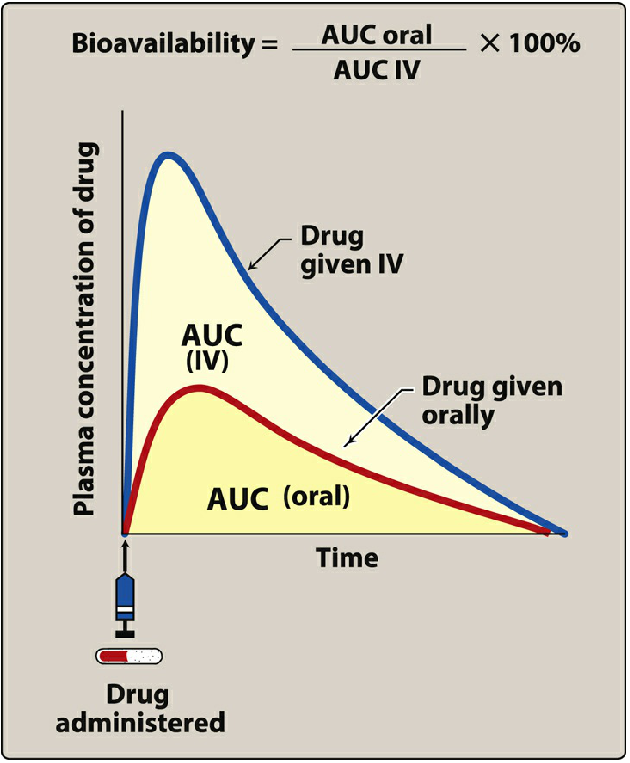
For orally administered drugs, only a fraction of the dose reaches the systemic circulation. This fraction (F) determines how the oral dose must be adjusted relative to the IV dose.
The core dose-conversion formula is:
Oral Dose = IV Dose / F
For example, if a drug has 50% oral bioavailability (F = 0.5) and the effective IV dose is 200 mg, the equivalent oral dose would be 200 / 0.5 = 400 mg.
2. Why Oral Bioavailability Differs from IV
Several factors reduce oral bioavailability, creating the central challenge of IV-to-PO conversion:
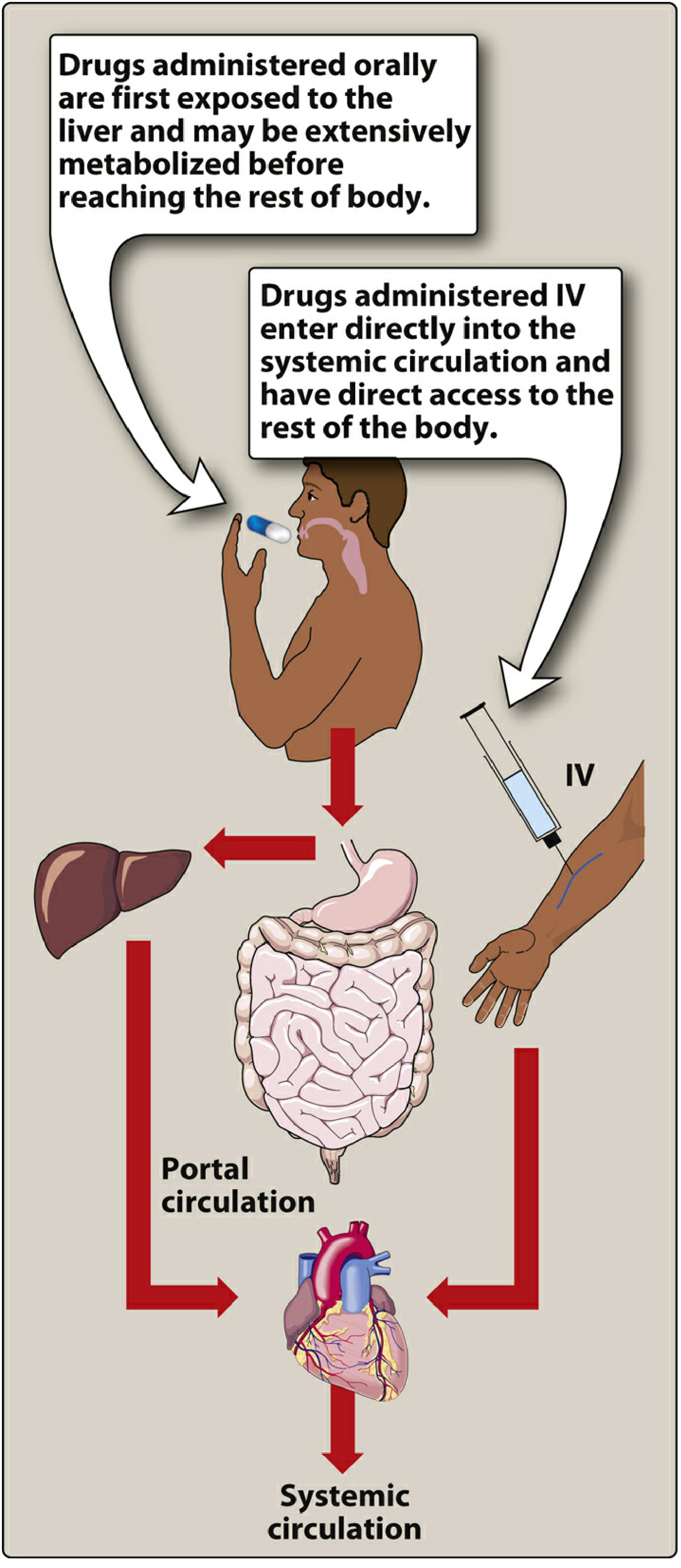
A. First-Pass Hepatic Metabolism
When an orally absorbed drug enters the portal circulation from the GI tract, it passes through the liver before reaching the systemic circulation. If the drug has a high hepatic extraction ratio, a large fraction is metabolized on this "first pass," drastically reducing the amount reaching the target tissues. (Lippincott Illustrated Reviews: Pharmacology, p. 41)
Classic examples:
- Nitroglycerin: >90% cleared during first-pass - primarily given sublingually, transdermally, or IV to bypass this effect
- Morphine: Significant first-pass glucuronidation - oral bioavailability is only ~25-35%, which is why oral morphine doses must be approximately 3× higher than parenteral morphine doses to achieve equianalgesic effect
- Propranolol: High extraction ratio; oral dose must be substantially larger than IV dose (Barash, Cullen, and Stoelting's Clinical Anesthesia, 9e)
Additionally, the small intestinal mucosal epithelium actively metabolizes drugs before they even reach the portal circulation, further reducing bioavailability. (Barash Clinical Anesthesia, p. 727)
B. Drug Solubility
- Very hydrophilic drugs cannot cross the lipid-rich cell membranes of the GI tract efficiently
- Very lipophilic drugs may be insoluble in aqueous GI fluids, limiting access to absorptive surfaces
- Optimal absorption requires a balance - drugs that are largely lipophilic with some aqueous solubility (often weak acids or weak bases) are best absorbed orally (Lippincott Illustrated Reviews: Pharmacology, p. 41)
C. Chemical Instability in the GI Tract
- Penicillin G is degraded by gastric acid - IV/IM formulation required; penicillin V (acid-stable) is the oral alternative
- Insulin is destroyed by GI proteolytic enzymes - must be administered parenterally
- Aminoglycosides (gentamicin, tobramycin) are not absorbed orally at all - IV/IM only for systemic infections
D. Drug Formulation Factors
Particle size, salt form, crystal polymorphism, enteric coatings, and excipients (binders, disintegrants) all affect dissolution rate and absorption. (Lippincott Illustrated Reviews: Pharmacology, p. 41)
E. Gastric Emptying Variability
The small intestine - with its enormous surface area - is the primary site of drug absorption. Since gastric emptying rate determines when drug reaches this absorptive surface, any delay (e.g., food, illness, opioids, diabetic gastroparesis) makes oral absorption highly variable and unpredictable. This is why oral dosing is generally impractical intraoperatively. (Barash Clinical Anesthesia, p. 727)
3. Criteria for IV-to-Oral Conversion
A patient is generally suitable for oral step-down therapy when:
| Clinical Criterion | Rationale |
|---|---|
| Hemodynamic stability | Adequate GI perfusion for absorption |
| Resolution of fever / improving clinical signs | Infection or condition responding to therapy |
| Ability to swallow / functional GI tract | No vomiting, ileus, or GI malabsorption |
| Tolerating oral fluids/feeds | Gastric emptying is functional |
| Drug available in oral form | With adequate bioavailability for the indication |
| No indication requiring rapid plasma levels | Oral route has delayed and variable Tmax |
For infections specifically, the key question is whether the organism is susceptible to an oral agent that achieves adequate tissue concentrations - not just adequate plasma concentrations.
4. Drug-Specific Conversion Considerations
A. High-Bioavailability Drugs (Near 1:1 IV-to-PO Conversion)
These drugs are the best candidates for direct step-down at equivalent doses:
| Drug | Oral Bioavailability | Notes |
|---|---|---|
| Fluoroquinolones (ciprofloxacin, levofloxacin, moxifloxacin) | ~85-99% | Gold standard for oral step-down in infections |
| Metronidazole | ~90-100% | IV and oral equally effective once tolerating PO |
| Fluconazole | ~90% | 1:1 IV-to-oral conversion; linear pharmacokinetics |
| Linezolid | ~100% | Full IV-equivalent oral dosing possible |
| Voriconazole | ~90% (adults) | Step-down feasible in adults once clinically stable; bioavailability can be as low as 60% in children, requiring TDM (Tietz Textbook of Laboratory Medicine, 7e) |
| Doxycycline | ~93% | Near-identical IV and oral dosing |
| Clindamycin | ~90% | Reliable step-down for skin/soft tissue infections |
B. Low-Bioavailability Drugs (Require Dose Increase at Step-Down)
When oral bioavailability is substantially less than 100%, the oral dose must be proportionally increased:
| Drug | Oral Bioavailability | IV-to-PO Conversion |
|---|---|---|
| Morphine | ~25-35% | Oral dose ~3× the IV/parenteral dose |
| Hydromorphone | ~20-35% | Oral dose ~5× the parenteral dose |
| Oxycodone | ~60-87% | ~1.5× more potent than oral morphine |
| Verapamil | ~20-35% | Significant first-pass effect |
| Propranolol | ~25-30% | Oral dose must be considerably higher |
| Tacrolimus | ~20-25% | Therapeutic drug monitoring (TDM) essential |
C. Drugs with No Adequate Oral Form
These drugs cannot be converted to oral therapy and must remain parenteral for systemic use:
- Aminoglycosides (gentamicin, amikacin) - not orally absorbed
- Vancomycin - oral form only works for C. difficile colitis (local GI effect); no systemic absorption
- Beta-lactams with poor oral bioavailability (e.g., piperacillin-tazobactam, meropenem, cefepime)
- Amphotericin B
5. Opioid Equianalgesic Conversion (Clinical Example)
Pain management provides the clearest and most clinically practiced application of IV-to-PO conversion. The following equianalgesic dose table is used when rotating or switching opioids and routes:
(Table 132.2, Sleisenger and Fordtran's Gastrointestinal and Liver Disease)
| Drug | Oral/Rectal Route | Parenteral Route | Key Conversion Principle |
|---|---|---|---|
| Morphine sulfate | 30 mg PO | 10 mg IV/SC | Parenteral morphine is 3× more potent than oral |
| Hydromorphone | 7 mg PO | 1.5 mg IV | Parenteral ~20× more potent than oral morphine |
| Oxycodone | 20 mg PO | N/A | Oral oxycodone ~1-1.5× more potent than oral morphine |
| Hydrocodone | 20 mg PO | N/A | Similar potency to oral morphine |
The oral route is the preferred route for opioid administration on the basis of availability, cost, and ease of use. (Sleisenger and Fordtran's GI Disease, p. 3692)
When switching to oral therapy, it is standard practice to also provide a breakthrough dose of 10-20% of the total 24-hour opioid dose for rescue analgesia.
6. Clinical Significance of IV-to-PO Conversion
A. Cost Reduction
IV drug formulations are almost universally more expensive than their oral equivalents. IV administration also requires nursing time, IV tubing, pumps, and regular site care. Prompt step-down to oral therapy produces substantial cost savings per patient per hospital stay.
B. Patient Safety
- Eliminates catheter-related complications: bloodstream infections (CLABSI), phlebitis, thrombosis, and infiltration
- Reduces exposure to IV-related errors (rate programming errors, incompatibility)
- Promotes earlier patient mobilization (no IV line attachment)
C. Hospital Stay Reduction
Oral step-down therapy is a key trigger for discharge eligibility in many conditions (pneumonia, cellulitis, urinary tract infection). Patients who can tolerate oral medications and are clinically stable may be safely discharged to complete their course at home, freeing hospital beds and reducing nosocomial infection exposure.
D. Antimicrobial Stewardship
In infectious diseases, protocols for IV-to-oral switch are a cornerstone of antimicrobial stewardship programs (ASPs). Using high-bioavailability oral antibiotics (fluoroquinolones, metronidazole, trimethoprim-sulfamethoxazole) eliminates the need for prolonged IV antibiotic courses, reducing selection pressure for resistant organisms and venous access complications.
E. Therapeutic Drug Monitoring (TDM) at Step-Down
For narrow therapeutic index drugs (e.g., tacrolimus, voriconazole, warfarin, digoxin), conversion from IV to oral requires careful monitoring of plasma drug levels, since bioavailability may vary between patients and change the effective dose. Voriconazole exemplifies this - high bioavailability in most adults permits routine step-down, but variable absorption in children mandates TDM. (Tietz Textbook of Laboratory Medicine, 7e, p. 1766)
7. Summary of the Conversion Process
1. Assess clinical readiness for step-down
   (hemodynamic stability, tolerating PO, functional GI tract)
         ↓
2. Identify the drug's oral bioavailability (F)
         ↓
3. Calculate equivalent oral dose:
   Oral Dose = IV Dose ÷ F
         ↓
4. Confirm oral formulation is appropriate
   (no crushing of extended-release; no NG tube incompatibility)
         ↓
5. Adjust dosing interval if needed
   (oral Tmax is delayed; dosing frequency may change)
         ↓
6. Monitor for therapeutic equivalence and adverse effects
   (TDM for narrow therapeutic index drugs)
Key references:
- Lippincott Illustrated Reviews: Pharmacology (pp. 40-41) - bioavailability and first-pass metabolism
- Barash, Cullen, and Stoelting's Clinical Anesthesia, 9e (p. 727) - oral administration pharmacokinetics
- Sleisenger and Fordtran's GI and Liver Disease (pp. 3692-3701) - opioid equianalgesic conversion table
- Tietz Textbook of Laboratory Medicine, 7e (p. 1766) - voriconazole IV-to-PO step-down
What are nomograms? Explain their applications in pharmacokinetic studies with examples. Give their advantages and disadvantages.
Finding Sources
Finding Sources
Finding Sources
Finding Sources
Finding Sources
Finding Sources
Reading File
Finding Sources
Reading File
Reading File
Loading Image
Finding Sources
Finding Sources
Finding Sources
Reading File
Searching the Web
nomogram pharmacokinetics applications advantages disadvantages drug dosing
I now have a thorough body of textbook evidence and can compile a comprehensive, well-cited answer.
Nomograms: Definition, Pharmacokinetic Applications, and Evaluation
1. What is a Nomogram?
A nomogram (from Greek: nomos = law, gramma = writing) is a two-dimensional graphical calculating instrument that encodes a mathematical relationship between three or more variables. It is constructed so that a straight line - or a plotted point - connecting known values on two scales automatically yields the correct answer on a third scale, without requiring direct calculation by the user.
In the context of pharmacokinetics, nomograms encode complex multi-variable equations (such as those governing drug clearance, half-life, dosing intervals, and toxicity thresholds) into a single visual diagram, allowing rapid, bedside estimation that would otherwise require logarithmic computation or computer software.
The three structural types of nomograms are:
- Alignment (parallel-scale) nomograms - three parallel (or angled) scales where a straight line connecting two known values intersects the third scale at the answer
- Cartesian/graphical nomograms - use x-y axes with plotted zones (e.g., the Rumack-Matthew nomogram)
- Proportion-based nomograms - scaled differently for subpopulations (e.g., pediatric body surface area charts)
2. Pharmacokinetic Foundations Underlying Nomograms
Nomograms in pharmacokinetics encode the following relationships:
| Parameter | Relationship Encoded |
|---|---|
| Bioavailability (F) | F = AUC(oral) / AUC(IV) × 100% |
| Creatinine Clearance | CrCl = [(140 - Age) × Weight] / [72 × SCr] (×0.85 for women) |
| Half-life (t½) | t½ = 0.693 / Ke |
| Volume of distribution (Vd) | Vd = Dose / C₀ |
| Steady-state concentration | Css = (F × Dose) / (CL × τ) |
| Toxicity probability | Log[Drug concentration] vs. time after ingestion |
Each nomogram simplifies one or more of these into a visual format.
3. Applications of Nomograms in Pharmacokinetic Studies
Application 1: The Rumack-Matthew Nomogram (Acetaminophen Toxicity)
The most widely used pharmacokinetic nomogram in emergency medicine is the Rumack-Matthew nomogram, which determines whether a patient with an acetaminophen (paracetamol) overdose requires antidotal treatment with N-acetylcysteine (NAC).
How it works:
- A serum acetaminophen concentration is measured at a known time after ingestion
- This single data point (concentration vs. time) is plotted on the semilogarithmic graph
- The nomogram is divided into three risk zones: No Risk, Possible Risk, and Probable Risk
- The decision line was originally set at 200 mcg/mL at 4 hours, then conservatively lowered to 150 mcg/mL at 4 hours to increase the safety margin for treatment decisions
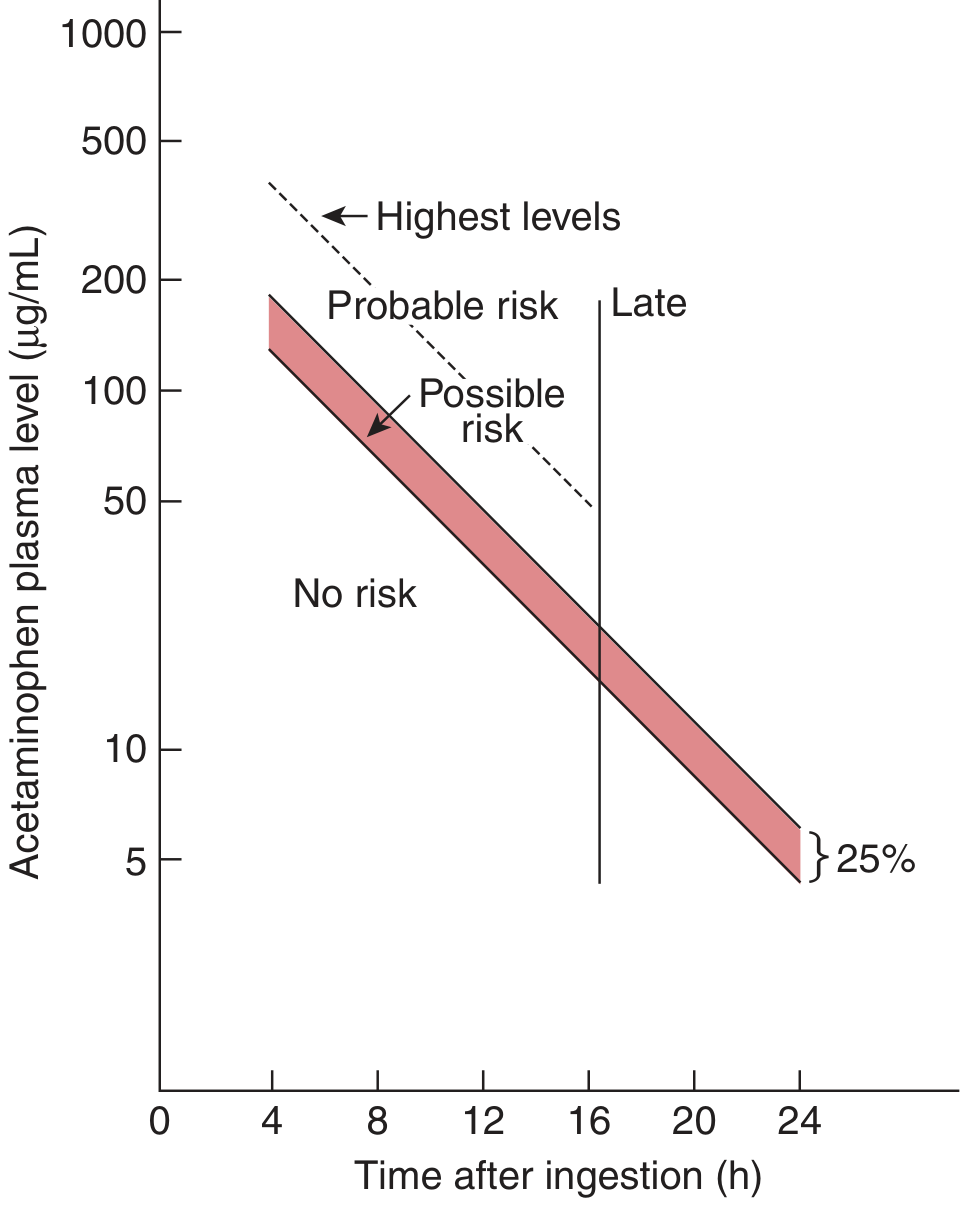
Pharmacokinetic basis: Acetaminophen follows predictable first-order elimination kinetics after a single oral overdose, so the plasma concentration falls along a straight line on a semilog graph - making a time-concentration plot the ideal nomographic format.
Clinical outputs from the nomogram:
- Concentrations above the "possible risk" line at any given time point → treat with NAC
- Below the "no risk" line → antidotal treatment unnecessary
- Patients above the "probable risk" (original) line at 4 hours had a 60% risk of hepatotoxicity and 5% mortality (Tintinalli's Emergency Medicine, p. 1129)
Validated qualifications and limitations (Tietz Textbook of Laboratory Medicine, 7e, p. 3566):
- Blood must be drawn no earlier than 4 hours after ingestion (to ensure absorption is complete)
- Valid only for single acute ingestions - not for chronic or repeated ingestions
- Cannot be used if time of ingestion is unknown
- If absorption is delayed (e.g., co-ingested anticholinergic drug), the concentration plotted may underrepresent actual toxicity
- In alcoholic, fasting, malnourished, or enzyme-induced patients (e.g., chronic phenobarbital use), the decision line may need to be lowered by 50-70%
Application 2: Aminoglycoside Dosing Nomograms (Hartford Nomogram)
Aminoglycosides (gentamicin, tobramycin, amikacin) have a narrow therapeutic index, with toxicity (nephrotoxicity, ototoxicity) linked to trough concentrations and time above a threshold, while efficacy is concentration-dependent (linked to peak:MIC ratio). Dosing nomograms allow precise individualization without repeated sampling.
Types of nomograms used:
(a) Traditional Dosing Nomograms
For thrice-daily or twice-daily dosing:
- Serum creatinine-based nomograms encode the Cockcroft-Gault formula to relate creatinine clearance to dose interval adjustments
- Input: patient's serum creatinine and weight
- Output: recommended dose interval (e.g., every 8h, 12h, or 24h)
"Nomograms and formulas have been constructed relating serum creatinine levels to adjustments in traditional treatment regimens." (Katzung's Basic and Clinical Pharmacology, 16e, p. 1288)
Therapeutic monitoring targets for traditional dosing:
- Peak levels: 5-10 mcg/mL (8-10 mcg/mL for serious infections)
- Trough levels: <2 mcg/mL (above this threshold is predictive of toxicity) (Katzung's, p. 1288)
(b) Extended-Interval / Once-Daily Dosing Nomogram (Hartford Nomogram)
Once-daily dosing exploits aminoglycoside concentration-dependent killing and post-antibiotic effect while minimizing toxicity:
- A standard dose of 5-7 mg/kg (gentamicin/tobramycin) or 15 mg/kg (amikacin) is given once daily
- Serum concentration is measured 6-14 hours after the dose
- This single data point is plotted on the Hartford nomogram
- The nomogram divides outcomes into zones labeled q24h, q36h, or q48h - indicating the appropriate redosing interval to maintain efficacy while avoiding toxic trough accumulation
- The goal is: drug concentrations <1 mcg/mL between 18-24 hours post-dose, allowing drug "washout" before the next dose (Katzung's Basic and Clinical Pharmacology, 16e, p. 1368)
"Several nomograms have been developed and validated to assist clinicians with once-daily dosing (eg, Freeman reference, Hartford nomogram)." (Katzung's Basic and Clinical Pharmacology, 16e)
Practical advantages of once-daily nomograms:
- Repeated serum concentration checks are unnecessary unless treatment extends >3 days
- Less labour-intensive; compatible with outpatient therapy
- Safer - total time above the toxic trough threshold is less with a single large dose than with multiple small doses (Katzung's, p. 1287)
Application 3: Renal Dose Adjustment Nomograms
For any renally-cleared drug (aminoglycosides, vancomycin, digoxin, methotrexate, lithium, NSAIDs, most antibiotics), nomograms encode the Cockcroft-Gault formula or GFR-based adjustments:
Variables on the scales:
- Age, body weight, serum creatinine
- Output: estimated CrCl or recommended dose fraction
Example construction (Cockcroft-Gault):
CrCl = [(140 - Age) × Weight (kg)] / [72 × Serum Creatinine (mg/dL)] (×0.85 for women)
A three-scale alignment nomogram encodes this equation: connect a point on the "age" scale to a point on the "serum creatinine" scale - the straightedge intersects the "CrCl" scale at the estimated clearance value. Separate curves are provided for males and females.
Application 4: Body Surface Area (BSA) Nomograms
Mosteller, DuBois, or Boyd BSA nomograms are used in:
- Oncology: chemotherapy dosing (virtually all cytotoxic agents are dosed in mg/m²)
- Pediatric dosing
- Cardiovascular drug dosing
Variables:
- Height (cm or inches) on one scale
- Weight (kg or lb) on a second scale
- BSA (m²) read off the central scale
BSA (m²) = √[Height (cm) × Weight (kg) / 3600]
The nomogram visually encodes this equation: a straight line connecting the height and weight scales intersects the BSA scale at the correct value. In chemotherapy, dose = BSA × drug dose in mg/m².
Application 5: Digoxin Dosing Nomogram
Digoxin has an extremely narrow therapeutic index (therapeutic range: 0.5-2 ng/mL; toxicity above 2 ng/mL). Nomograms for digoxin dosing incorporate:
- Lean body weight (digoxin distributes in lean tissue, not fat)
- Renal function (CrCl) - the primary determinant of digoxin clearance
- Age - renal function and volume of distribution both change with aging
Output: recommended loading dose and maintenance dose, with suggested intervals for level monitoring.
Application 6: Phenobarbital/Barbiturate Withdrawal Supplementary Dosing Nomogram
Used for patients undergoing barbiturate withdrawal protocols, nomograms encode a loading dose calculation based on the degree of dependence and target phenobarbital concentration, simplifying what would otherwise require multiple sequential calculations. (Brenner and Rector's The Kidney, 2-Volume Set)
Application 7: Voriconazole and Antifungal TDM
For antifungals like voriconazole, nomograms can integrate plasma drug concentrations, timing after dose, and clinical status to guide:
- Whether the current dose is adequate (above the minimum effective concentration)
- Whether dose reduction is needed to prevent neurotoxicity or hepatotoxicity
High oral bioavailability (~90%) in adults allows IV-to-oral step-down, but pediatric patients show variable absorption as low as 60%, requiring TDM - nomograms incorporating trough concentration + time assist in interpreting results. (Tietz Textbook of Laboratory Medicine, 7e, p. 1766)
4. Advantages of Nomograms
| Advantage | Explanation |
|---|---|
| Speed | Instantaneous - no calculation required at the bedside; decisions can be made in seconds |
| Simplicity | Encodes complex multi-variable equations into a single visual tool accessible to all healthcare providers |
| No calculator needed | Especially valuable in resource-limited settings, emergencies, or power-failure scenarios |
| Reduces arithmetic errors | Eliminates transcription and computation mistakes that can occur with manual formula application |
| Visual clarity | Risk zones (e.g., treat / don't treat in Rumack-Matthew) are immediately visible; clinicians see relationships rather than just numbers |
| Validated population data embedded | Represent data from large clinical outcome studies (e.g., the Rumack-Matthew nomogram is based on thousands of overdose cases) |
| Facilitates individualization | Patient-specific variables (age, weight, serum creatinine) are inputted to yield individualized outputs rather than population averages |
| Standardizes practice | Reduces inter-clinician variability in dosing and treatment decisions |
| Applicable across skill levels | Nurses, pharmacists, and physicians can all use nomograms without advanced pharmacokinetic training |
5. Disadvantages and Limitations of Nomograms
| Disadvantage | Explanation |
|---|---|
| Static - cannot account for all variables | Built from fixed population datasets; cannot account for individual variation in drug metabolism, genetic polymorphisms, or organ function changes |
| Not valid outside their defined scope | The Rumack-Matthew nomogram applies only to single acute oral ingestions between 4-24 hours; applying it outside this context risks under- or over-treating |
| Require accurate input data | Garbage in = garbage out: an inaccurate time of ingestion, incorrect weight, or erroneous serum creatinine will produce a wrong answer |
| Do not replace TDM | For narrow therapeutic index drugs (vancomycin, aminoglycosides, digoxin, tacrolimus), nomograms provide an initial estimate - therapeutic drug monitoring (actual plasma level measurement) remains necessary |
| Population-specific | A nomogram validated for adults may not apply to pediatric, pregnant, critically ill, or obese patients without modification |
| Risk of false security | Clinicians may over-rely on the nomogram output without considering the full clinical picture |
| Two-dimensional limitation | Traditional nomograms can only visualize 3 variables. For drugs with complex multi-compartment kinetics or numerous covariates (e.g., vancomycin), pharmacokinetic software and Bayesian estimation are superior |
| Cannot account for drug interactions | Enzyme inducers/inhibitors alter clearance in ways that nomograms do not capture |
| Graphical reading error | Reading a line on a printed scale introduces human error in the form of interpolation imprecision |
| Outdated in the digital era | Pharmacokinetic software (e.g., DoseMeRx, MwPharm, InsightRx) using Bayesian individualization has largely superseded nomograms for complex dosing in tertiary care settings |
6. Summary
| Feature | Detail |
|---|---|
| Definition | Graphical calculator encoding multi-variable pharmacokinetic equations |
| Core principle | Connecting known values on aligned scales yields unknown values |
| Best-known example | Rumack-Matthew nomogram (acetaminophen toxicity) |
| Other examples | Hartford nomogram (aminoglycosides), BSA nomograms (chemotherapy), renal dose-adjustment nomograms, digoxin dosing |
| Strength | Speed, simplicity, validated population data, standardization |
| Weakness | Static, population-based, limited to scope of derivation, cannot replace TDM |
Key references:
- Katzung's Basic and Clinical Pharmacology, 16e (pp. 1287-1288) - aminoglycoside nomograms and Hartford nomogram
- Tintinalli's Emergency Medicine (pp. 1127-1143) - Rumack-Matthew nomogram
- Tietz Textbook of Laboratory Medicine, 7e (pp. 3560-3570) - Rumack-Matthew nomogram (figure) and voriconazole TDM
- Lippincott Illustrated Reviews: Pharmacology (pp. 40-41) - bioavailability and AUC relationships
- Brenner and Rector's The Kidney, 2-Volume Set - barbiturate withdrawal supplementary dosing nomogram
Describe the principle of superposition and how it applies to multiple drug dosing.
Finding Sources
Finding Sources
Finding Sources
Finding Sources
Finding Sources
Finding Sources
Reading File
Reading File
Reading File
Reading File
Reading File
Loading Image
Loading Image
Finding Sources
Loading Image
Finding Sources
Reading File
Finding Sources
Finding Sources
I now have comprehensive textbook content and figures. Let me write the complete answer.
The Principle of Superposition and Multiple Drug Dosing
1. The Principle of Superposition - Definition
The principle of superposition is a fundamental concept in pharmacokinetics that states:
In a linear (first-order) pharmacokinetic system, the total drug concentration in the body at any point in time during a multiple-dosing regimen is equal to the arithmetic sum of the residual concentrations contributed by each individual dose still present in the body at that moment.
In other words, each dose behaves as if it were administered into a "drug-free" body - independently of all preceding doses. The contributions of all doses simply add together (superimpose) to produce the total observed plasma concentration. This is only valid when drug behavior is linear - meaning the pharmacokinetic parameters (clearance, volume of distribution, half-life) remain constant regardless of the drug concentration present.
The principle originates from the superposition theorem in mathematics and physics: in any linear system, the response to a set of simultaneous inputs equals the sum of the individual responses to each input applied alone.
2. Prerequisites: Linear (First-Order) Pharmacokinetics
Superposition holds only under linear pharmacokinetic conditions:
| Feature of Linear PK | Explanation |
|---|---|
| First-order elimination | A constant fraction of drug is eliminated per unit time (not a constant amount) |
| Dose-proportional AUC | Doubling the dose doubles the AUC and Cmax |
| Constant half-life | t½ does not change with dose or accumulated concentration |
| Constant clearance | Enzymatic elimination is not saturated at therapeutic concentrations |
| Constant Vd | Tissue binding sites are not saturated |
Most drugs at therapeutic concentrations follow first-order (linear) kinetics, making superposition applicable to the vast majority of clinical dosing scenarios.
Exceptions - nonlinear (zero-order / Michaelis-Menten) kinetics break superposition:
- Phenytoin: Elimination enzymes saturate within the therapeutic range. Small dose increases produce disproportionately large rises in plasma concentration
- Ethanol, aspirin (at high doses): Metabolic saturation
- These drugs cannot be predicted by simple superposition
3. Mathematical Expression of Superposition
For a drug given as n equal IV bolus doses (each dose D) administered at equal intervals (τ), the concentration at any time t after the n-th dose is:
C(t) = C₁(t) + C₁(t - τ) + C₁(t - 2τ) + ... + C₁(t - [n-1]τ)
Where:
- C₁(t) = the concentration at time t after a single dose
- Each subsequent term represents the residual concentration from each of the previous doses, each shifted in time by one dosing interval
This can be written more compactly as:
C(t) = C₁(t) × [1 - e^(-n·Ke·τ)] / [1 - e^(-Ke·τ)]
Where:
- Ke = first-order elimination rate constant = 0.693 / t½
- n = number of doses administered
- τ = dosing interval
As n → ∞ (i.e., as dosing continues), this simplifies to the steady-state equation:
C_ss(t) = C₁(t) / [1 - e^(-Ke·τ)]
The term 1 / (1 - e^(-Ke·τ)) is the accumulation factor - it tells you how much larger the steady-state concentration is compared to the first-dose concentration.
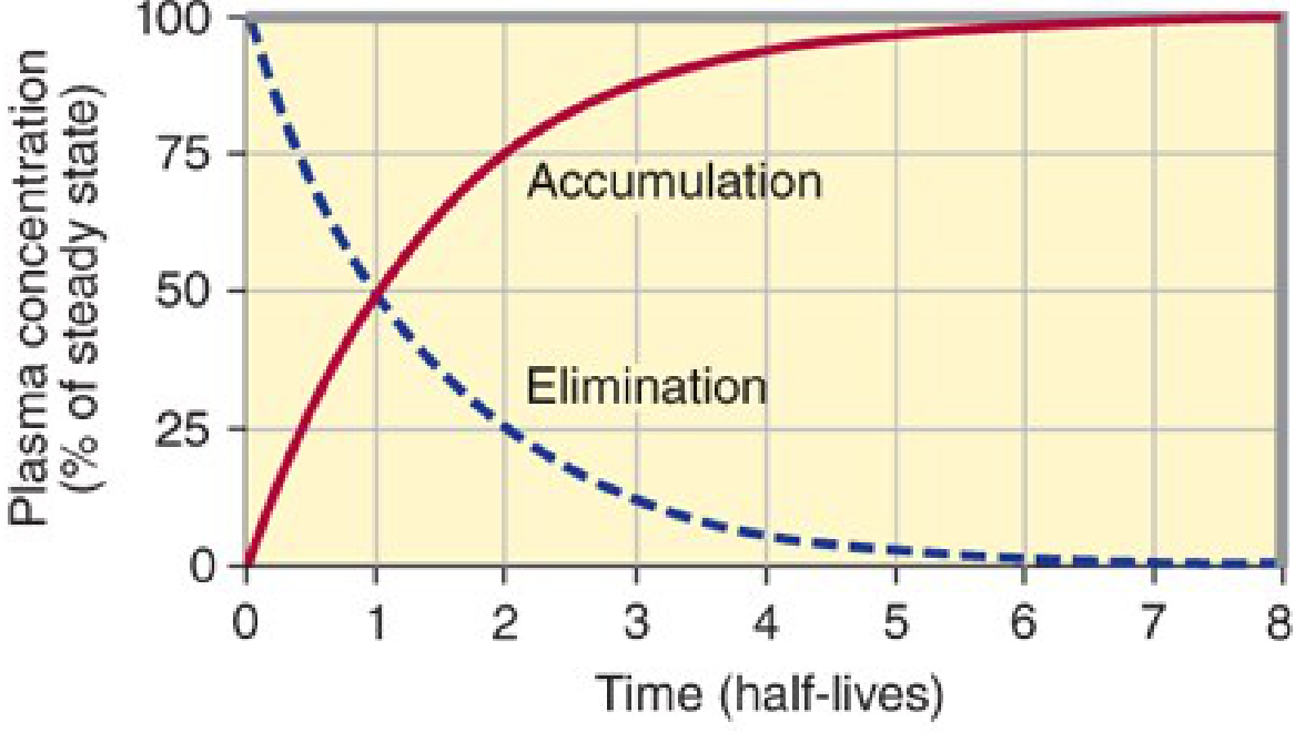
4. Drug Accumulation: The Practical Result of Superposition
Because it theoretically takes infinite time to completely eliminate a dose, whenever the dosing interval is shorter than complete elimination, residual drug from each prior dose remains when the next dose is given. The doses successively layer on top of one another - they superimpose - causing drug accumulation until a steady state is reached.
(Katzung's Basic and Clinical Pharmacology, 16e, p. 1715)
"Whenever drug doses are repeated, the drug will accumulate in the body until dosing stops. This is because it takes an infinite time (in theory) to eliminate all of a given dose. In practical terms, this means that if the dosing interval is shorter than four half-lives, accumulation will be detectable."
5. Step-by-Step Illustration of Superposition
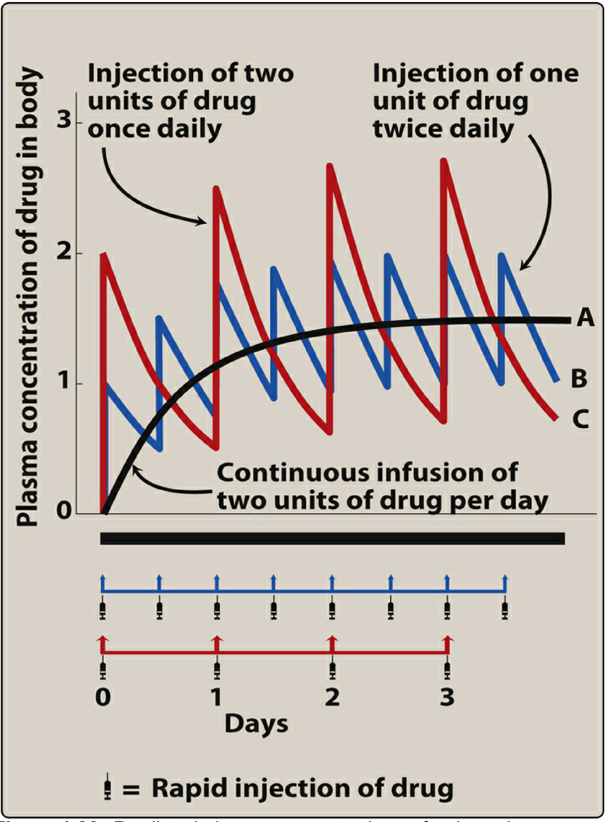
Example: Drug with t½ = 1 day, administered IV once daily (dose = 1 unit)
| End of Dosing Interval | Residual from Dose 1 | Residual from Dose 2 | Total (Trough) | Peak after next dose |
|---|---|---|---|---|
| After Dose 1 | 0.50 units remaining | - | 0.50 units | 1.50 (after D2) |
| After Dose 2 | 0.25 units | 0.50 units | 0.75 units | 1.75 (after D3) |
| After Dose 3 | 0.125 | 0.25 | 0.375 = 0.875 trough | 1.875 (after D4) |
| Steady state | ... | ... | → 1.00 unit trough | → 2.00 units peak |
(Lippincott Illustrated Reviews: Pharmacology, p. 70)
"The minimal amount of drug remaining during the dosing interval progressively approaches a value of 1.00 unit, whereas the maximal value immediately following drug administration progressively approaches 2.00 units. Therefore, at the steady state, 1.00 unit of drug is lost during the dosing interval, which is exactly matched by the rate of administration. That is, the 'rate in' equals the 'rate out.'"
This is the principle of superposition in action - each dose's concentration-time profile is summed with all preceding residuals to produce the total concentration at each moment.
6. Steady State
Steady state is defined as the condition in which rate of drug input = rate of drug elimination, so that drug concentrations fluctuate between a reproducible peak (Cmax,ss) and trough (Cmin,ss) within every dosing interval.
(Maudsley Prescribing Guidelines, 15e, p. 890)
"Repeated dosing of any drug that is not completely removed within the dosing interval will inevitably lead to accumulation... Eventually, a point is reached where blood levels remain stable within a specific peak-to-trough range - this is steady state."
Time to Reach Steady State
The time to reach steady state depends only on the drug's half-life, not on the dose or dosing frequency:
| Number of Half-Lives | % Steady State Reached |
|---|---|
| 1 | 50% |
| 2 | 75% |
| 3 | 87.5% |
| 4 | 94% |
| 5 | 97% |
(Maudsley Prescribing Guidelines, 15e)
~4-5 half-lives are needed to reach practically useful steady state. This is a direct mathematical consequence of superposition - each dose's residual adds to the total, following a geometric series that converges at steady state.
Key relationship: Steady State and Accumulation Factor
Accumulation factor = 1 / (1 - e^(-0.693 × τ/t½))
(Katzung's Basic and Clinical Pharmacology, 16e, p. 1719)
For a drug dosed once every half-life: accumulation factor = 1 / (1 - 0.5) = 2
This means the steady-state peak concentration is exactly twice the first-dose peak - the superimposition of doses doubles the plateau compared to the first-dose level when τ = t½.
7. Practical Applications to Multiple Drug Dosing
A. Effect of Dosing Frequency at the Same Daily Dose
Superposition predicts that splitting a daily dose into smaller, more frequent doses:
- Does not change the mean steady-state concentration (Css,avg) - the total daily dose and clearance determine this
- Does not change the time to reach steady state
- Does reduce peak-to-trough fluctuation (smaller swings around the mean)
"Using smaller doses at shorter intervals reduces the amplitude of fluctuations in drug concentration. However, the dosing frequency changes neither the magnitude of Css nor the rate of achieving Css." (Lippincott Illustrated Reviews: Pharmacology, p. 621)
B. Loading Dose
When a rapid therapeutic effect is needed (e.g., arrhythmia, severe infection), waiting 4-5 half-lives for steady state via superposition is too slow. A loading dose is used to immediately fill the volume of distribution to the target steady-state level:
Loading dose = Vd × Target Css / F
A loading dose does not change the time course of subsequent accumulation - steady state is still reached at 4-5 half-lives via superposition of maintenance doses. The loading dose simply shifts the entire accumulation curve upward to the target level from the start.
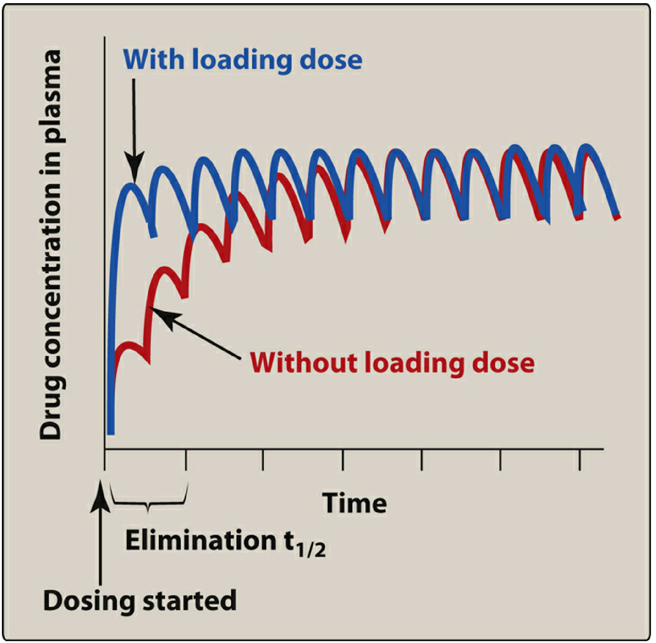
(Lippincott Illustrated Reviews: Pharmacology, p. 645)
"Loading doses do not hasten the achievement of steady state levels." (Maudsley Prescribing Guidelines, 15e, p. 1959)
C. Maintenance Dose Design
The maintenance dose is calculated to replace exactly what is lost in each dosing interval (the superposition "rate-in = rate-out" equilibrium):
Dosing rate = Target Css × CL / F
Where CL = clearance and F = bioavailability.
Superposition ensures that if the correct maintenance dose is selected, the plasma concentration will accumulate in a predictable pattern and stabilize at the target steady-state range.
D. Dose Adjustment in Organ Impairment
Superposition allows prediction of new steady-state concentrations when clearance changes (e.g., renal failure reduces aminoglycoside CL):
- If CL is halved, superposition predicts that Css will double at the same dosing rate
- Dose or interval must be adjusted to restore the original steady-state target
8. When Superposition Breaks Down
The principle fails when pharmacokinetics are nonlinear (dose-dependent):
| Scenario | Mechanism | Drug Examples |
|---|---|---|
| Enzyme saturation | Elimination rate cannot increase further at high concentrations; approaches zero-order | Phenytoin, ethanol, aspirin (high dose) |
| Protein binding saturation | As binding sites fill, free drug fraction rises disproportionately | Valproate at high doses |
| Transporter saturation | Efflux or uptake transporters become saturated | Methotrexate |
| Autoinduction | Drug induces its own metabolism over time, reducing levels | Carbamazepine |
| Time-dependent pharmacokinetics | Clearance changes over the course of treatment | Some antiretrovirals |
In these cases, predicting steady-state concentrations from first-dose data using superposition is unreliable, and therapeutic drug monitoring becomes essential.
9. Summary Table
| Concept | Application of Superposition |
|---|---|
| Drug accumulation | Each dose adds to residuals from all prior doses until steady state |
| Steady state | Rate-in = Rate-out; reached after ~4-5 t½ regardless of dose or frequency |
| Accumulation factor | Ratio of Css to C-after-first-dose = 1/(1-e^(-0.693×τ/t½)) |
| Dosing frequency effect | Affects peak-trough fluctuation, not mean Css or time to Css |
| Loading dose | Achieves target level instantly; does not alter time to true steady state |
| Dose adjustment | Proportional relationship between dose and Css (linear systems only) |
| Limitations | Fails with nonlinear kinetics (phenytoin, ethanol, protein-saturated drugs) |
Key references:
- Katzung's Basic and Clinical Pharmacology, 16e (pp. 1715-1730) - drug accumulation, accumulation factor, half-life
- Lippincott Illustrated Reviews: Pharmacology (pp. 614-659) - fixed-dose regimens, steady state, loading dose
- The Maudsley Prescribing Guidelines in Psychiatry, 15e (pp. 890-891) - steady state and timing of sampling
Explain in detail pharmacokinetic/ pharmacodynamics correlation in drug therapy.
Your credits are exhausted. You can purchase a top-up or subscribe to a plan to continue using Orris. If you're already subscribed, your daily credits will reset tomorrow.
This is a shared conversation. Sign in to Orris to start your own chat.