Scatter radiation its formation and control : beam centering devices , obligatory, cone diaphragm and grids in detail
scatter radiation formation production Compton interaction radiography
beam centering devices collimator cone diaphragm aperture diaphragm scatter control radiography
scatter radiation grid radiography diagram
antiscatter grid Bucky grid ratio grid lines per centimeter radiographic quality
scatter radiation Compton effect primary beam fog image contrast degradation kVp
Scatter Radiation: Formation, Effects & Control
1. What Is Scatter Radiation?
2. Formation of Scatter Radiation
2.1 Mechanisms of X-ray Interaction with Matter
| Interaction | Energy Range | Scatter Produced? | Relevance |
|---|---|---|---|
| Coherent (Rayleigh) scattering | < 30 keV | Yes (no energy loss) | Minimal clinical relevance |
| Compton scattering | 30 keV – 30 MeV | Yes (main source) | Primary scatter mechanism in diagnostic radiology |
| Photoelectric absorption | < 100 keV | No | Creates contrast, no scatter |
| Pair production | > 1.02 MeV | Indirect | Not relevant at diagnostic energies |
2.2 Compton Scattering in Detail
- An incoming X-ray photon collides with an outer-shell (loosely bound) electron.
- The photon transfers part of its energy to the electron, ejecting it (Compton recoil electron).
- The photon is deflected at a new angle with reduced energy — this is the scatter photon.
- The ejected electron ionizes surrounding tissue — contributing to biological dose.
- Scatter can travel in any direction, including back toward the tube (backscatter) and toward the detector.
- The angle of deflection depends on the energy transferred; higher energy photons scatter more in the forward direction.
- Scatter photons carry no useful diagnostic information — they expose the detector at random positions, creating fog (uniform gray veiling glare) that reduces image contrast.
2.3 Factors That Increase Scatter Production
| Factor | Effect on Scatter |
|---|---|
| Higher kVp | Increases proportion of Compton interactions; more scatter |
| Larger field size (FOV) | More tissue volume irradiated → more scatter photons |
| Greater tissue thickness | More interactions → more scatter |
| Higher atomic number of tissue | Minor effect; Compton depends on electron density, not Z |
| Absence of beam restriction | Maximizes irradiated volume |
3. Effects of Scatter on Image Quality
- Reduced contrast: Scatter photons strike the image receptor diffusely, adding a uniform background density (fog) that "washes out" the subject contrast differential.
- Reduced signal-to-noise ratio (SNR): Scatter is noise; more scatter = lower SNR.
- Reduced spatial resolution: Diffuse distribution of scatter blurs edge definition.
- Increased patient dose: Scatter within tissues contributes directly to absorbed dose.
- Occupational radiation hazard: Scatter exiting the patient is the main source of staff dose — following the inverse square law, exposure drops as 1/d² with distance from the patient (Radiation Safety, p. 28).
4. Control of Scatter Radiation
- Reduce scatter production — limit the volume of tissue irradiated (beam-restricting devices)
- Reduce scatter reaching the detector — intercept scatter after it is produced (grids, air gaps)
5. Beam-Centering and Beam-Restricting Devices
5.1 Aperture Diaphragm (Simple Diaphragm)
- A flat lead (Pb) plate with a fixed, pre-cut rectangular or circular opening placed at the tube port.
- Restricts the X-ray beam to the size of the aperture cutout.
- Beam centering is achieved by aligning the aperture with the tube's central ray.
- Simple, cheap, robust.
- No moving parts.
- Fixed field size — cannot be adjusted without changing the plate.
- Penumbra (geometric unsharpness) at field edges because the diaphragm has finite thickness and is close to the focal spot.
- Not suitable when different anatomical regions or variable field sizes are needed.
5.2 Cone and Cylinder Diaphragm
- A hollow cone or cylinder of lead-lined metal attached to the tube housing exit port.
- May be fixed or interchangeable.
| Type | Shape | Field Shape Produced |
|---|---|---|
| Flared cone | Diverges outward | Circular, large coverage |
| Straight cylinder | Uniform diameter | Circular, more restricted |
| Extension cylinder | Long cylinder | Very small, highly restricted circular field |
- The inner walls of the cone/cylinder absorb off-axis primary radiation and scatter originating within the cone itself.
- Limits the beam to a circular field at the detector.
- Provides additional scatter cleanup compared to a flat diaphragm because photons must travel the length of the cone to reach the film — scattered photons are absorbed by the walls.
- The central ray of the beam must align with the long axis of the cone/cylinder.
- Centering lights or laser localizers are used to align the cone to the part.
- Better scatter reduction than a flat diaphragm (cone walls absorb oblique scatter).
- Simple, inexpensive.
- Lightweight for portable use.
- Circular field is not matched to rectangular image receptors — corners of the film are unexposed (wasted dose potential to ensure coverage).
- Cannot restrict field to irregular shapes.
- Fixed dimensions limit flexibility.
5.3 Variable-Aperture Collimator (Light-Beam Diaphragm / Multi-Leaf Collimator)
- Contains two pairs of lead shutters (one pair for each axis — longitudinal and transverse) arranged at right angles to each other, plus an optional iris diaphragm for fine adjustment.
- A light bulb and mirror system projects a visible light field onto the patient that exactly matches the X-ray field at the focal-film distance (FFD/SID).
- The light enables precise pre-exposure field centering and sizing.
- Both shutter pairs can be independently adjusted to produce any rectangular field size.
- By adjusting shutter pairs, field can be varied from near-zero to the maximum field size.
- Light-beam indicator allows precise beam centering to the area of interest before exposing the patient.
- Fully adjustable field size — can be tailored to any anatomy.
- Visual verification of field position before exposure (light beam).
- Most effective scatter reduction of all beam-limiting devices (rectangular field fits image receptor).
- Reduces patient dose by minimizing irradiated tissue.
- Collimators should always be visible within the field of view (Cardiac Catheterization, p. 43).
- Must be correctly calibrated — light field must align within ±2% of SID with the actual X-ray field.
- More expensive than cones/diaphragms.
- Requires regular QA testing.
- Collimation reduces the volume of tissue exposed, spares surrounding organs, reduces DAP (dose-area product), and reduces scatter at the detector — improving contrast and enabling visualization of fine structures such as stents (Cardiac Catheterization, p. 43).
5.4 Summary Comparison: Beam-Restricting Devices
| Device | Field Shape | Adjustable? | Scatter Reduction | Visual Centering |
|---|---|---|---|---|
| Aperture diaphragm | Fixed (rect/circ) | No | Minimal | No |
| Cone/cylinder | Circular | No | Moderate | No (use centering light) |
| Variable collimator | Rectangular | Yes | Best | Yes (light beam) |
6. Grids — Detailed
6.1 Principle of Grid Action
- The primary beam travels in a straight line from the focal spot to the detector.
- Scatter photons travel in oblique, random directions.
- A grid consists of alternating radiopaque lead strips and radiolucent interspace material oriented parallel (or angled) to the primary beam path.
- Lead strips intercept the obliquely traveling scatter photons; primary beam photons (traveling in the correct direction) pass through the interspaces.
6.2 Grid Construction
| Component | Material | Function |
|---|---|---|
| Lead strips (septa) | Pure lead (Pb) | Absorb scatter photons |
| Interspace material | Aluminum, carbon fiber, or organic fiber | Allow primary beam transmission; provide structural support |
| Cover plates | Aluminum | Structural protection |
6.3 Grid Parameters
a) Grid Ratio (r)
| Grid Ratio | Scatter Cleanup | Primary Transmission | Use |
|---|---|---|---|
| 5:1 | Low | High | Pediatrics, low kVp |
| 8:1 | Moderate | Moderate | General radiography |
| 10:1 | Good | Moderate | Chest, abdomen |
| 12:1 | High | Lower | High kVp, thick parts |
| 16:1 | Very high | Lowest | Very high kVp |
b) Grid Frequency (Lines per cm / lines per inch)
- Number of lead strip pairs per unit distance.
- Typical range: 25–60 lines/cm (60–150 lines/inch).
- Higher frequency → thinner strips → less visible grid lines on image → better image quality.
- Low-frequency grids may produce visible grid lines on the radiograph (Moire effect with digital systems).
c) Grid Focus
| Type | Description | Use |
|---|---|---|
| Parallel (non-focused) | All lead strips are vertical/parallel | Short SIDs, small grids, portable |
| Focused | Lead strips angled to converge toward a focal point at a specified focal distance | Standard radiography at a defined SID |
| Cross-hatch (crossed) | Two focused or parallel grids at 90° | Maximum scatter cleanup; no movement possible |
d) Focal Range (Focused Grids)
- A focused grid is designed for a specific focal distance and focal range.
- Using a focused grid outside its focal range causes grid cutoff — peripheral loss of primary beam transmission.
6.4 Grid Types by Movement
| Type | Description | Effect on Image |
|---|---|---|
| Stationary grid | Fixed in position during exposure | Grid lines visible on image |
| Moving grid (Potter-Bucky / Bucky grid) | Grid oscillates during exposure | Grid lines blurred out (invisible on final image) |
- Introduced by Gustav Bucky (1913) and refined by Hollis Potter.
- The grid moves perpendicular to the lead strips during the exposure, blurring the grid lines.
- Movement speed must be synchronized with exposure time to ensure complete line blurring.
- The Bucky is now the standard component of radiographic tables and upright stands.
- Bucky factor = ratio of incident radiation to transmitted radiation = measure of how much dose must be increased to compensate for grid absorption.
6.5 Grid Selectivity and Efficiency Measures
| Measure | Formula | Meaning |
|---|---|---|
| Primary transmission (Tp) | Primary passing through / Primary incident | What fraction of useful beam reaches receptor |
| Scatter transmission (Ts) | Scatter passing through / Scatter incident | What fraction of scatter still reaches receptor |
| Selectivity (Σ) | Tp / Ts | Ratio of primary to scatter transmission — higher is better |
| Contrast improvement factor (K) | Contrast with grid / Contrast without grid | Practical measure of grid benefit |
| Bucky factor (B) | Total incident / Total transmitted | Compensatory exposure increase needed |
6.6 Grid Cutoff
| Cause | Pattern of Cutoff |
|---|---|
| Off-center (lateral decentering) | Uniform density loss across whole film |
| Off-focus (wrong SID for focused grid) | Peripheral density loss, bilateral |
| Off-level (grid tilted) | Unilateral density loss on one side |
| Upside-down focused grid | Severe peripheral density loss, central clear |
| Combination | Complex, mixed pattern |
6.7 Indications for Grid Use
| Body Part Thickness | kVp | Grid Needed? |
|---|---|---|
| < 10 cm | Any | Usually No (use air-gap instead) |
| 10–15 cm | < 60 kVp | Optional |
| > 15 cm | Any | Yes |
| Any | > 80 kVp | Recommended |
6.8 Alternatives to Grids
| Method | Mechanism | Best For |
|---|---|---|
| Air-gap technique | Scatter diverges and misses detector due to increased OID | Angiography, magnification, pediatrics |
| Beam restriction (collimation) | Reduces volume of scatter production | Always used as primary method |
| Low kVp | Shifts toward photoelectric (no scatter) | When contrast is priority |
| Digital post-processing | Software scatter correction | Digital detectors |
7. Practical Hierarchy of Scatter Control
1. Restrict the beam (collimate to the smallest clinically adequate field)
        ↓
2. Optimize kVp (use lowest kVp consistent with diagnostic quality)
        ↓
3. Reduce tissue volume (compression where appropriate)
        ↓
4. Use a grid (when tissue > 10–15 cm or high kVp)
        ↓
5. Increase distance from patient (staff protection — inverse square law)
8. Key Takeaways
- Compton scattering is the dominant mechanism producing scatter in diagnostic radiography; it increases with higher kVp and larger field sizes.
- Beam-restricting devices (diaphragms → cones → variable collimators) reduce scatter by limiting the irradiated volume; the light-beam collimator is the most versatile and effective.
- Cones and cylinders provide circular field restriction with moderate scatter cleanup; useful where small, focused beams are required.
- Grids intercept scatter after production; grid ratio, frequency, focus, and movement type determine scatter cleanup efficiency and image quality.
- The Bucky (moving grid) eliminates visible grid lines from the radiograph.
- Grid cutoff is a critical quality control concern with focused grids — correct SID and centering are mandatory.
- All beam restriction methods reduce both patient dose and scatter simultaneously — they are complementary, not alternatives.
Beam centering devices ? In control of scatter radiation
beam centering devices scatter radiation control radiography collimator diaphragm cone cylinder
beam restricting devices collimator cone diaphragm radiography scatter control
beam limiting devices field size collimation scatter reduction radiographic technique
light beam collimator variable aperture diaphragm X-ray beam restriction
collimation field size scatter production primary beam restriction patient dose reduction image contrast
collimation effect on scatter radiation image quality radiograph
Beam Centering Devices in the Control of Scatter Radiation
Why Beam Centering Devices Control Scatter
"Collimation uses metallic apertures within the X-ray source to modify the beam and minimise the radiation field size to the required area of interest… collimation not only produces sharper images by hardening the beam, but also reduces radiation exposure to the patient and medical personnel." — Radiation Safety, p. 21
Smaller field size  →  Less irradiated tissue volume
                    →  Fewer Compton interactions
                    →  Less scatter produced
                    →  Less fog on image  →  Better contrast
                    →  Less dose to patient and staff
Classification of Beam-Centering Devices
Beam-Centering / Beam-Limiting Devices
│
├── 1. Aperture Diaphragm (Fixed)
├── 2. Cone and Cylinder Diaphragm
└── 3. Variable-Aperture Collimator (Light-Beam Diaphragm)
1. Aperture Diaphragm
Structure
- A flat sheet of lead (Pb) with a single fixed opening (rectangular, circular, or square) mounted at the exit port of the X-ray tube housing.
- The opening is precisely sized for a specific projection and film size at a given FFD (focus-film distance).
How It Controls Scatter
- Allows only the photons passing through the aperture opening to proceed toward the patient.
- All photons outside the aperture boundaries are absorbed by the lead plate before they even reach the patient.
- By preventing irradiation of surrounding tissue, it eliminates scatter that would otherwise be produced in those regions.
Diagram (Schematic)
X-ray Tube
     │
     ▼
 [Lead Plate]
 ┌──────────┐
 │          │  ← Lead absorbs photons outside aperture
 │  [HOLE]  │  ← Aperture opening
 │          │
 └──────────┘
     │
     ▼
 Primary beam (restricted)
     │
   Patient
Beam Centering
- The central ray of the X-ray beam must be aligned with the center of the aperture hole.
- Since the field size is fixed, the tube must be precisely positioned — no adjustment is possible at the device level.
Characteristics
| Feature | Detail |
|---|---|
| Field shape | Fixed (rectangular or circular) |
| Adjustability | None |
| Scatter reduction | Basic — limits field but no oblique photon cleanup |
| Penumbra | Present — lead plate is close to the focal spot |
| Cost | Very low |
| Complexity | Minimal |
Advantages
- Simple, durable, inexpensive
- No mechanical parts to fail
- Lightweight — suitable for portable units
Disadvantages
- Cannot be adjusted — different plates needed for different field sizes
- No visual preview of field on patient (no light beam)
- Circular/square openings may not match rectangular image receptors
- Does not eliminate oblique off-axis primary radiation as effectively as longer devices
Clinical Use
- Dental intraoral X-ray units
- Simple portable radiographic units
- Situations where a fixed, reproducible field is always required
2. Cone and Cylinder Diaphragm
Structure
| Form | Shape | Characteristic |
|---|---|---|
| Cone (flared) | Diverges outward (trumpet shape) | Larger circular field at the patient |
| Cylinder (extension tube) | Uniform diameter throughout | Smaller, highly restricted circular field |
How It Controls Scatter
- The entry end of the cone limits the beam to a defined area, restricting irradiated tissue volume.
- The length of the device creates a "channeling" effect.
- Any photon traveling obliquely (not along the central axis) will strike the lead-lined inner walls and be absorbed.
- This is more effective than a flat plate because scattered photons generated within the proximal part of the cone are also absorbed before exiting.
X-ray Tube
     │
  [Entry]
  ┌────┐
  │    │  ← Narrow opening restricts beam
  │    │  ← Walls absorb oblique photons
  │    │
  └────┘
  (Cylinder or flared cone)
     │
     ▼
 Restricted circular field
     │
   Patient
Effect of Cone Length on Scatter Control
Short cone:   [==]     → Less restriction, more scatter passes
Long cylinder: [======] → Maximum restriction, oblique photons eliminated
Beam Centering
- The central ray must align with the long axis of the cone/cylinder.
- Misalignment causes the beam to strike the inner walls, creating a cone-cut artifact — partial or complete loss of density on one side of the image.
- Centering aids used:
- External centering ring/locator on the patient end
- Separate centering light or laser device
- Alignment markers
Cone-Cut Artifact
Correct alignment:        Cone-cut (misalignment):
 ┌──────────┐              ┌──────────┐
 │██████████│              │████░░░░░░│
 │██ Image ██│              │████  CUT │
 │██████████│              │████░░░░░░│
 └──────────┘              └──────────┘
  Full density              Loss of density on one side
Characteristics
| Feature | Detail |
|---|---|
| Field shape | Circular |
| Adjustability | None (interchangeable sets) |
| Scatter reduction | Moderate–good (wall absorption adds benefit over flat diaphragm) |
| Risk of artifact | Cone-cut if misaligned |
| Cost | Low |
Advantages
- Better scatter reduction than a flat aperture diaphragm
- Simple, no moving parts
- Wall absorption removes oblique scatter within the cone
- Lightweight sets available
Disadvantages
- Circular field does not match rectangular image receptors — corners of film/detector are unexposed
- Fixed field size — different cones needed for different areas
- Longer cylinders can be cumbersome
- Cone-cut artifact with poor centering
- No light-beam preview of field on patient (unless a separate light system is used)
Clinical Use
- Dental periapical radiography (long cylinder is standard)
- Skull and sinus radiography
- Cephalometry
- Fluoroscopic spot coning
- Any application requiring a small, well-defined circular field
3. Variable-Aperture Collimator (Light-Beam Diaphragm / Multi-Leaf Collimator)
Structure
X-ray Tube (Focal Spot)
         │
   ┌─────┴─────┐
   │  Primary  │ ← Primary collimator (fixed; limits maximum field)
   │ diaphragm │
   └─────┬─────┘
         │
   ┌─────┴─────────────────┐
   │  Pair 1: Lead Shutters │ ← Controls field width (X-axis)
   │   ◄──────────────►    │
   └─────┬─────────────────┘
         │
   ┌─────┴─────────────────┐
   │  Pair 2: Lead Shutters │ ← Controls field length (Y-axis)
   │        ▲              │
   │        ▼              │
   └─────┬─────────────────┘
         │
   ┌─────┴─────┐
   │   Mirror  │ ← Reflects light from bulb
   │   + Bulb  │ ← Projects light field onto patient
   └─────┬─────┘
         │
         ▼
   Light field on patient = exact replica of X-ray field
Components in Detail
| Component | Material/Type | Function |
|---|---|---|
| Primary (fixed) collimator | Lead | Defines maximum possible beam size |
| Shutter Pair 1 | Lead leaves | Adjusts beam width independently |
| Shutter Pair 2 | Lead leaves | Adjusts beam length independently |
| Mirror | Half-silvered glass at 45° | Reflects light along X-ray path |
| Light bulb | Positioned at mirror level | Simulates focal spot position |
| Filter slot | Aluminum | Added beam filtration |
| Cover glass | Borosilicate | Protects internal components |
How It Controls Scatter
-
Primary restriction: The two independently adjustable pairs of lead shutters confine the X-ray beam to exactly the area of clinical interest — no more, no less.
-
Rectangular field: Matches the shape of the image receptor, minimizing wasted irradiation.
-
Precise centering: The light beam projects the exact field on the patient before the exposure, allowing the radiographer to:
- Confirm correct anatomy is included
- Confirm surrounding structures are excluded
- Minimize field size while maintaining diagnostic coverage
-
Maximum scatter reduction: Of all beam-limiting devices, a correctly adjusted variable collimator produces the smallest clinically adequate field — meaning the minimum scatter for the task.
Beam Centering — The Light Beam Advantage
Step 1: Position patient
Step 2: Adjust shutters → light field projected onto patient skin
Step 3: Visually confirm field covers area of interest ONLY
Step 4: Adjust shutters further if needed (fine-tune exclusion of unnecessary anatomy)
Step 5: Expose — X-ray field is identical to light field
Scatter Reduction: Effect of Field Size
| Field Size | Scatter Fraction (approximate, 80 kVp, 20 cm tissue) |
|---|---|
| 5 × 5 cm | ~20% |
| 10 × 10 cm | ~40% |
| 20 × 20 cm | ~60% |
| 35 × 35 cm (open field) | ~80% |
Characteristics
| Feature | Detail |
|---|---|
| Field shape | Rectangular (adjustable to any size) |
| Adjustability | Fully variable (continuous adjustment) |
| Scatter reduction | Best of all beam-limiting devices |
| Visual centering | Yes — light-beam preview |
| Alignment risk | Minimal — visual confirmation prevents errors |
| Cost | Highest |
| Maintenance | Requires periodic QA calibration |
Advantages
- Adjustable to any field size within limits
- Rectangular field matches image receptors (no wasted corners)
- Light beam enables precise, confirmed beam centering
- Best scatter reduction → best image contrast → lowest patient dose for task
- Universally standardized on modern X-ray equipment
Disadvantages
- Most expensive of the three device types
- Requires calibration and QA testing
- Light bulb can fail — must be checked before use
- Mirror angle can shift — requires periodic verification
- Heavier than cones/diaphragms
Clinical Use
- All modern fixed radiographic rooms (tables, upright stands)
- Fluoroscopy units
- Angiography suites
- Mobile radiographic units (modern versions)
- Mandatory on all general-purpose diagnostic X-ray equipment
4. Comparison Summary — All Three Devices
| Feature | Aperture Diaphragm | Cone / Cylinder | Variable Collimator |
|---|---|---|---|
| Field shape | Fixed (rect/circ) | Circular only | Rectangular (any size) |
| Adjustable? | No | No | Yes |
| Visual field preview | No | No | Yes (light beam) |
| Scatter reduction | Basic | Moderate | Best |
| Centering accuracy | Poor (no feedback) | Moderate (risk of cone-cut) | Excellent |
| Matches film/detector? | Partially | No (circular vs rectangular) | Yes |
| Cost | Very low | Low | High |
| Complexity | None | Minimal | Moderate |
| Best for | Fixed-field portable use | Dental, small-field skull | All general radiography |
5. General Principle: How All These Devices Reduce Scatter
Reduce the irradiated tissue volume → reduce the number of Compton interactions → reduce the number of scatter photons produced → reduce fog on the image → improve contrast → reduce patient and staff dose.
6. Clinical Rule
Always collimate to the smallest field that includes all diagnostically necessary anatomy. Overcollimation (excluding needed anatomy) requires repeat exposure and doubles patient dose. Undercollimation (open field) maximizes scatter, degrades the image, and irradiates tissue unnecessarily. The correct balance is achieved by using the light-beam variable collimator as the primary tool, guided by anatomical landmarks before every exposure.
In my topic for dexa for exam point of view as Msc radiology student what to add give me step by step answer more effectively
DEXA dual energy X-ray absorptiometry bone mineral density osteoporosis
PMID: 39316095
DEXA scan DXA bone densitometry spine hip scan image
DEXA (DXA) — Complete MSc Radiology Exam Notes
Step-by-step structure covering every examinable point from basic physics through clinical interpretation, artifacts, and recent guidelines.
STEP 1 — Full Name, Definition & Historical Context
- Preceded by Single Photon Absorptiometry (SPA) and Dual Photon Absorptiometry (DPA) — both used radioactive isotopes (iodine-125, gadolinium-153), limiting precision and requiring long scan times.
- DXA introduced in the 1980s, replacing radioisotope sources with an X-ray tube — revolutionizing the diagnosis and monitoring of osteoporosis.
- Currently the WHO-endorsed gold standard for BMD measurement.
STEP 2 — Physical Principle (The Core Exam Topic)
2.1 The Dual-Energy Principle
| Beam | Energy | Preferentially attenuated by |
|---|---|---|
| High energy (H) | ~100–140 kVp | Soft tissue (lower differential for bone) |
| Low energy (L) | ~40–70 kVp | Bone (higher photoelectric absorption due to calcium) |
2.2 How Two Energies Are Produced
- A cerium (Ce) or samarium (Sm) filter with a K-edge in the relevant energy range shapes the beam spectrum.
- Single exposure; filter selectively absorbs photons in one energy range.
- The X-ray tube rapidly alternates between high kVp (~100 kV) and low kVp (~40 kV) pulses.
- Separate detector readings at each pulse are processed independently.
STEP 3 — Equipment & System Design
3.1 Types of DXA Systems
| System Type | X-ray Beam | Scan Method | Speed | Precision |
|---|---|---|---|---|
| Pencil-beam (1st gen) | Single pencil beam | Rectilinear point-by-point scan | Slow (10–30 min) | Moderate |
| Fan-beam (current standard) | Wide fan beam | Single sweep across body | Fast (30 sec–5 min) | High |
| Narrow fan-beam | Intermediate | Compromise between above | Moderate | High |
- Much faster scan times → reduced motion artifact
- Higher spatial resolution
- Allows vertebral fracture assessment (VFA) in the same session
- Magnification artifact — objects closer to the tube appear larger (affects accuracy in obese patients)
3.2 DXA Machine Components
X-ray Tube (alternating kVp)
        ↓
   Beam filtration
        ↓
   Patient on scan table
        ↓
   Detector array (C-arm sweeps over patient)
        ↓
   Analog-to-digital converter
        ↓
   Computer analysis software
        ↓
   BMD maps + T/Z scores + printed report
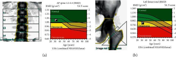
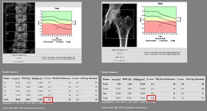
STEP 4 — Scan Sites (Regions of Interest)
4.1 Primary Sites
| Site | Region Measured | Why Important |
|---|---|---|
| Lumbar spine (L1–L4) | PA or AP view | High trabecular bone content → sensitive to early change; reflects axial skeletal status |
| Proximal femur (hip) | Femoral neck + total hip | Best predictor of hip fracture risk; used for WHO classification |
| Distal 1/3 radius (forearm) | Non-dominant arm | Used when spine/hip not measurable; reflects cortical bone |
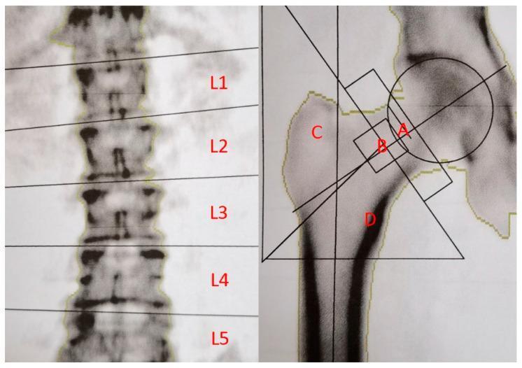
4.2 Proximal Femur Sub-Regions
| Region | Description |
|---|---|
| A — Femoral neck | Narrow cortical band; most critical for fracture prediction |
| B — Ward's triangle | Junction of three trabecular groups; lowest BMD area; no longer used for diagnosis |
| C — Greater trochanter | Primarily cancellous bone |
| D — Intertrochanteric shaft | Cortical-rich region |
| Total hip | Sum of all regions; most reproducible |
4.3 Additional/Specialist Sites
| Site | Indication |
|---|---|
| Lateral spine (L2–L4) | Excludes posterior element artifacts; less used due to poor precision |
| Whole body | Body composition analysis (fat mass, lean mass, BMC) |
| Forearm only | Hyperparathyroidism, bilateral hip replacements, extreme obesity |
| Pediatric DXA | AP spine + whole body (not hip); Z-scores used exclusively |
| Vertebral Fracture Assessment (VFA) | Lateral spine imaging in same session using fan-beam |
STEP 5 — Output Measurements
5.1 Primary Outputs
| Measurement | Units | Definition |
|---|---|---|
| BMC (Bone Mineral Content) | grams (g) | Total mineral mass in scanned region |
| Area | cm² | Projected 2D area of scanned bone |
| BMD (Bone Mineral Density) | g/cm² | BMC ÷ Area (areal density — not true volumetric density) |
Critical exam point: DXA measures areal BMD (g/cm²), NOT volumetric BMD. This is a known limitation — larger bones appear denser even with the same volumetric density (size artifact).
5.2 T-Score
- Compares patient's BMD to a young healthy adult reference population (peak bone mass)
- Used for diagnosis of osteoporosis in postmenopausal women and men ≥ 50
| T-score | Diagnosis |
|---|---|
| > −1.0 | Normal |
| −1.0 to −2.5 | Osteopenia (low bone mass) |
| ≤ −2.5 | Osteoporosis |
| ≤ −2.5 + fragility fracture | Severe/established osteoporosis |
5.3 Z-Score
- Compares to an age-, sex-, and ethnicity-matched reference population
- Used for premenopausal women, men < 50, and children
- Z-score ≤ −2.0 = "below expected range for age" → secondary cause of bone loss must be investigated
| Score | Use |
|---|---|
| T-score | Postmenopausal women, men ≥ 50 |
| Z-score | Premenopausal women, men < 50, children, secondary osteoporosis |
STEP 6 — Indications for DXA
6.1 Clinical Indications (Exam List)
| Category | Specific Indication |
|---|---|
| Postmenopausal women | ≥ 65 years (universal); < 65 with risk factors |
| Men | ≥ 70 years; younger with risk factors |
| Fracture risk | History of fragility fracture; FRAX score suggests high risk |
| Secondary osteoporosis | Long-term glucocorticoid use (≥ 3 months) (Goldman-Cecil, p. 3995) |
| Disease-associated | RA, IBD, CKD, hyperparathyroidism, hypogonadism, anorexia nervosa, malabsorption |
| Drug monitoring | Androgen deprivation therapy, aromatase inhibitors, anticonvulsants |
| Monitoring therapy | Every 1–2 years during osteoporosis treatment (Washington Manual, p. 5728) |
| Body composition | Obesity surgery, sarcopenia, sports medicine |
| Children | Osteogenesis imperfecta, reduced bone density conditions (Grainger & Allison, p. 813) |
6.2 FRAX Integration
- Major osteoporotic fracture
- Hip fracture
- 10-year hip fracture risk ≥ 3%, OR
- 10-year major osteoporotic fracture risk ≥ 20% (Lippincott Pharmacology, p. 2644)
STEP 7 — Patient Preparation & Procedure
7.1 Pre-Scan Preparation
| Requirement | Detail |
|---|---|
| No barium/contrast | Avoid for 7–10 days (residual contrast absorbs X-rays falsely) |
| No nuclear medicine | Residual radioisotopes: wait 3–7 days depending on half-life |
| Remove metal objects | Jewellery, belts, zips, underwire bras — alter attenuation |
| Clothing | Light clothing without metal; gown if needed |
| Calcium supplements | Some protocols: hold 24 hrs before scan |
| Pregnancy | Contraindicated |
| Weight limit | Standard table limit ~204 kg; bariatric tables available |
| History | Note fractures, surgery, hardware — affects ROI selection |
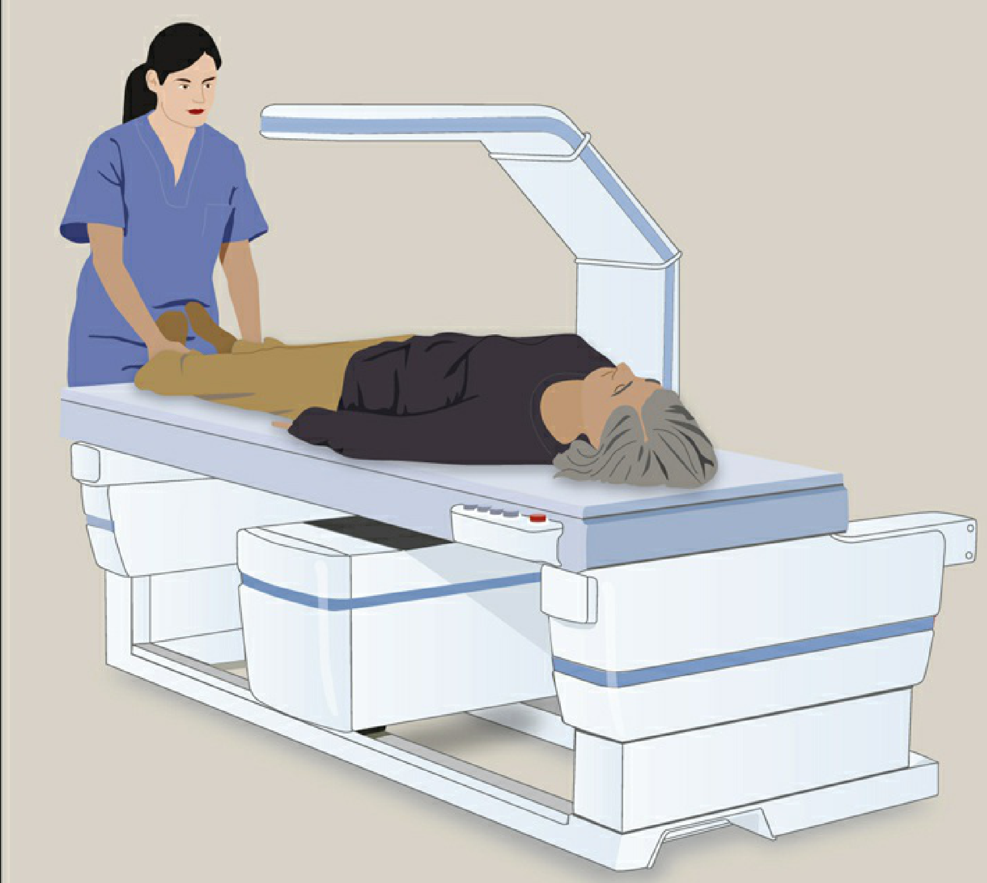
7.2 Patient Positioning
- Supine, arms at sides
- Hips and knees flexed ~90° over a positioning block → flattens lumbar lordosis, reduces posterior element overlap with vertebral bodies
- AP/PA direction
- Supine
- Foot internally rotated 15–25° using a positioning device → brings femoral neck parallel to table (removes neck anteversion artifact)
- Leg abducted slightly
- Opposite leg restrained
- Seated beside table, arm extended
- Non-dominant arm preferred
- Specific positioning device holds arm still
7.3 Scan Procedure (Fan-Beam)
- Patient positioned → technologist confirms alignment with positioning lasers
- Scout scan performed → software identifies scan region
- C-arm performs single sweep (30 sec – 5 min depending on site and system)
- Software auto-segments bone regions → technologist verifies and corrects ROI placement
- BMD values, T-scores, Z-scores automatically calculated and graphed
- Report generated and verified by reporting clinician/radiologist
STEP 8 — DXA Report Interpretation
8.1 Standard Report Contents
- Patient demographics (name, DOB, sex, ethnicity, weight, height)
- Scan date, machine manufacturer and model
- Scan sites imaged
- BMD (g/cm²), BMC (g), Area (cm²) for each region
- T-score and Z-score for each region
- Reference database used
- Graphic showing patient's BMD on age-normative curve
- Precision error / Least Significant Change (LSC)
- Clinical interpretation + comparison to prior scan
8.2 Graphical Output — Color-Coded BMD Curve
| Band Color | T-score Range | Classification |
|---|---|---|
| 🟢 Green | > −1.0 | Normal |
| 🟡 Yellow | −1.0 to −2.5 | Osteopenia |
| 🔴 Red | < −2.5 | Osteoporosis |
8.3 Monitoring — Least Significant Change (LSC)
- If BMD change < LSC → could be measurement error, not true biological change
- Typical spine precision: ~1%; LSC ≈ 2.77%
- Same scanner, same technologist, same positioning must be used for serial monitoring
STEP 9 — Vertebral Fracture Assessment (VFA)
- Lateral spine imaging (T4 to L4) in the same DXA session
- Identifies vertebral deformities and morphometric fractures that would otherwise require a separate spine X-ray
- Radiation dose much lower than conventional lateral spine radiograph (~3 µSv vs ~600 µSv)
- Used alongside BMD — vertebral fractures independently increase 10-year fracture risk
- Semi-quantitative grading (Genant scale):
| Grade | Deformity | % Height Loss |
|---|---|---|
| 0 | Normal | 0 |
| 1 | Mild | 20–25% |
| 2 | Moderate | 25–40% |
| 3 | Severe | > 40% |
STEP 10 — Body Composition by DXA
| Compartment | How Identified |
|---|---|
| Bone mineral | Dual-energy differential attenuation |
| Lean soft tissue | Soft tissue ROI minus fat tissue |
| Fat mass | Specific attenuation ratio of fat vs lean |
- Sarcopenia diagnosis (low lean mass + low function)
- Monitoring cancer cachexia, renal failure, HIV
- Sports science and athletic training
- Visceral fat estimation (android/gynoid distribution)
- Bariatric surgery outcome monitoring
STEP 11 — Radiation Dose
| Scan | Effective Dose (µSv) |
|---|---|
| DXA spine | ~1–3 µSv |
| DXA hip | ~1–5 µSv |
| VFA (lateral spine) | ~3–6 µSv |
| Whole body DXA | ~3–10 µSv |
| Chest X-ray (comparison) | ~20 µSv |
| Background radiation/day (comparison) | ~8 µSv/day |
| CT abdomen (comparison) | ~5,000–10,000 µSv |
STEP 12 — Artifacts & Sources of Error (High-Yield Exam Topic)
12.1 Causes of Falsely ELEVATED BMD (Overestimation)
| Cause | Mechanism |
|---|---|
| Vertebral osteophytes | Added mineral mass in scan field |
| Aortic calcification | Calcified aortic wall overlies vertebrae |
| Vertebral compression fracture | Compressed body = smaller area but same mineral → higher apparent density |
| Scoliosis | Rotated vertebrae overlap; abnormal ROI |
| Spinal hardware / metallic implants | Metal hyperattenuates beam |
| Hip prosthesis | Metal artifact at proximal femur |
| Residual barium contrast | Attenuates beam in GI tract |
| Obesity (fan-beam) | Magnification artifact |
| Clothing with metal | Zips, buttons, hooks |
| Patient movement | Motion artifact mimics density change |
12.2 Causes of Falsely REDUCED BMD (Underestimation)
| Cause | Mechanism |
|---|---|
| Laminectomy / spinal surgery | Removed posterior elements reduce measured bone |
| Incorrect patient positioning | Suboptimal ROI alignment |
| Patient rotation (spine) | Asymmetric projection of vertebra |
| Foot not internally rotated (hip) | Femoral neck not parallel → underestimation |
12.3 Precision Errors
- Repositioning error — slight differences in positioning between serial scans
- ROI placement variability — manual editing inconsistency
- Machine drift — requires daily phantom calibration to detect
- Software version changes — different algorithms give different values; must note software version
STEP 13 — Quality Control (QA)
| QA Measure | Frequency | Purpose |
|---|---|---|
| Spine phantom scan | Daily | Detect machine drift / calibration errors |
| Precision assessment | Per technologist | Calculate in-house LSC |
| Cross-calibration | When changing machines | Ensure continuity of serial data |
| Software version logging | Per report | Traceability |
| ISCD guidelines | Annual | International Society for Clinical Densitometry |
STEP 14 — Limitations of DXA
| Limitation | Clinical Impact |
|---|---|
| 2D projection (areal BMD, not volumetric) | Size bias — tall/large individuals score higher |
| Cannot distinguish trabecular from cortical bone | QCT superior for compartmental analysis |
| Artifacts elevate BMD in elderly | May miss true osteoporosis in patients with degenerative change |
| Cannot assess bone quality/microarchitecture | Only measures density, not structural competence |
| Population-specific reference databases needed | T-scores vary by ethnicity; non-Caucasian databases less well established |
| Cannot predict all fractures | Most fractures occur in osteopenic range due to larger population size |
| 2D cannot assess geometry | Hip structural analysis (HSA) needs additional software |
STEP 15 — Alternatives & Complementary Techniques
| Technique | Advantage over DXA | Disadvantage |
|---|---|---|
| QCT (quantitative CT) | Volumetric BMD; separates trabecular/cortical | Higher radiation dose; expensive |
| pQCT / HR-pQCT | Microarchitecture; peripheral sites | Research mainly; limited to radius/tibia |
| Quantitative Ultrasound (QUS) | No radiation; portable; cheap | Cannot be used for WHO diagnosis; poor precision |
| MRI | Trabecular microarchitecture; no radiation | Expensive; not routine |
| Radiogrammetry | Hand X-ray; measures cortical thickness | Limited to peripheral skeleton |
STEP 16 — Recent Guideline Update (Exam-Relevant 2025)
- Technical quality control procedures for the DXA instrument are critical for valid results.
- Patient positioning and ROI analysis approach significantly influence measurements.
- Selection of appropriate reference ranges for T-scores and Z-scores must be specified in every report.
- Non-BMD DXA measurements — particularly VFA — should be routinely integrated into clinical risk assessment.
- Reporting clinicians must have adequate knowledge of current interpretation standards to avoid errors.
STEP 17 — Quick Exam Summary Table
| Feature | Key Fact |
|---|---|
| Full name | Dual-Energy X-ray Absorptiometry |
| Gold standard for | BMD measurement and osteoporosis diagnosis |
| Two energies used | ~40–70 kVp (low) and ~100–140 kVp (high) |
| Main output | BMD in g/cm² (areal, not volumetric) |
| Primary scan sites | Lumbar spine (L1–L4), Proximal femur, 1/3 distal radius |
| T-score for osteoporosis | ≤ −2.5 (WHO) |
| T-score uses | Postmenopausal women, men ≥ 50 |
| Z-score uses | Premenopausal, men < 50, children |
| Radiation dose (spine) | ~1–3 µSv (extremely low) |
| Most common artifact | Osteophytes → falsely elevated lumbar BMD |
| Monitoring frequency | Every 1–2 years on treatment |
| Monitoring precision tool | Least Significant Change (LSC) = 2.77 × CV% |
| Key limitation | Areal density — size bias; cannot assess microarchitecture |
| VFA grading scale | Genant semi-quantitative (Grades 0–3) |
| 2025 Guideline (PMID) | 39316095 — Slart et al., EJNMMI |
- Lippincott Illustrated Reviews: Pharmacology, pp. 898–899
- The Washington Manual of Medical Therapeutics, p. 5728
- Goldman-Cecil Medicine, p. 3995
- Grainger & Allison's Diagnostic Radiology, p. 813
- Slart RHJA et al. Updated practice guideline for DXA. Eur J Nucl Med Mol Imaging 2025 Jan. [PMID: 39316095]
In my topic for dexa for exam point of view as Msc radiology student what to add give me step by step answer more effectively
DXA DEXA scan lumbar spine hip BMD T-score report graph
DXA dual energy absorptiometry bone mineral density clinical practice guideline
DEXA (DXA) — Complete MSc Radiology Exam Answer
✦ STEP 1 — Definition & Full Name
- Diagnosis of osteoporosis and osteopenia
- Fracture risk assessment
- Monitoring response to treatment
- Body composition analysis
✦ STEP 2 — Historical Background (Exam Context)
| Era | Technique | Limitation |
|---|---|---|
| 1960s | Single Photon Absorptiometry (SPA) | Radioactive source (¹²⁵I); peripheral sites only |
| 1970s | Dual Photon Absorptiometry (DPA) | Radioactive source (¹⁵³Gd); slow; source decays → imprecise |
| 1980s | DXA introduced | X-ray tube replaces isotope → stable, fast, precise |
| 1990s–now | Fan-beam DXA | Sub-minute scans; vertebral fracture assessment added |
✦ STEP 3 — Physical Principle (The Core Exam Topic)
3.1 The Beer-Lambert Law (Foundation)
3.2 Why Two Energies Solve This
3.3 Why Bone Attenuates More at Low Energy
- Bone mineral is primarily calcium hydroxyapatite [Ca₁₀(PO₄)₆(OH)₂]
- Calcium has a high atomic number (Z = 20) → strong photoelectric absorption at low kVp
- At low energy (~40–70 kVp): bone–soft tissue contrast is high
- At high energy (~100–140 kVp): both attenuate similarly → contrast is low
- The difference in these two attenuation values encodes the bone mineral content
3.4 Methods of Producing Two Energies
| Method | Mechanism | Used In |
|---|---|---|
| K-edge filtration | Cerium (Ce) or samarium (Sm) filter with K-edge at ~40 keV shapes the beam into two distinct energy peaks from a single exposure | Older/some current fan-beam systems |
| Voltage switching | X-ray tube rapidly alternates between high kVp (~100–140) and low kVp (~40–70) pulses; detector reads each separately | Most modern fan-beam systems |
✦ STEP 4 — Equipment Design
4.1 System Types
| Generation | Beam Type | Scan Method | Scan Time | Precision |
|---|---|---|---|---|
| 1st gen | Pencil beam | Point-by-point rectilinear scan | 20–30 min | Moderate |
| 2nd gen | Narrow fan beam | Sweep with small detector array | 5–10 min | Good |
| Current standard | Wide fan beam | Single sweep with wide detector array | 30 sec – 3 min | Excellent |
4.2 Machine Architecture
X-ray Tube (kVp alternating or filtered)
          ↓
    Beam collimation
          ↓
    Patient on table (supine)
          ↓
    C-arm sweeps over patient
          ↓
    Scintillation detector array (below table)
          ↓
    ADC + Computer software
          ↓
    BMD map → T/Z scores → printed report
4.3 Fan-Beam vs Pencil-Beam
| Feature | Pencil Beam | Fan Beam |
|---|---|---|
| Scan time | Long | Short |
| Spatial resolution | Lower | Higher |
| Motion artifact | More susceptible | Less susceptible |
| VFA possible? | No | Yes |
| Magnification artifact | Negligible | Present (diverging beam) |
| Radiation dose | Slightly lower | Slightly higher (still very low) |
✦ STEP 5 — Scan Sites and Positioning
5.1 Standard Primary Sites
| Site | Vertebrae / Region | Bone Type | Clinical Relevance |
|---|---|---|---|
| Lumbar spine | L1–L4 (AP/PA) | Rich trabecular bone | Sensitive to early metabolic change; high precision |
| Proximal femur | Femoral neck + total hip | Cortical + trabecular | Best predictor of hip fracture; WHO classification site |
| Distal 1/3 radius | Non-dominant arm | Predominantly cortical | Used when spine/hip not measurable |
5.2 Proximal Femur Sub-Regions (Know All Four)
| Label | Region | Note |
|---|---|---|
| A | Femoral neck | Narrow ROI; primary fracture prediction site |
| B | Ward's triangle | Intersection of 3 trabecular groups; lowest BMD; no longer used for diagnosis |
| C | Greater trochanter | Cancellous-rich |
| D | Intertrochanteric / shaft | Cortical-dominant |
| — | Total hip | Sum of above; most reproducible; preferred for monitoring |
5.3 Positioning Protocol (Exam-Critical)
- Supine, arms folded on chest
- Hips and knees flexed ~90° over a foam positioning block → flattens lumbar lordosis → reduces posterior element (spinous process, facets) overlap with vertebral bodies → accurate anterior body measurement
- Supine, leg extended
- Foot internally rotated 15–25° using a foot-holder → brings femoral neck parallel to table → removes anteversion artifact → accurate neck measurement
- Slight abduction of the hip
- Seated beside table
- Non-dominant arm extended, palm down
- Positioning device immobilizes arm
- ROI at 33% (one-third) site from wrist
✦ STEP 6 — Output Measurements (What DXA Produces)
6.1 Primary Outputs
| Output | Unit | Formula |
|---|---|---|
| BMC (Bone Mineral Content) | grams (g) | Directly measured |
| Area | cm² | Projected 2D area of bone |
| BMD (Bone Mineral Density) | g/cm² | BMC ÷ Area |
Critical exam point — DXA limitation: DXA measures areal BMD (2D projection), not true volumetric BMD (g/cm³). A larger bone will appear denser than a smaller bone with identical volumetric density. This is the size artifact — a key weakness of DXA.
6.2 T-Score
- Compares to peak bone mass (healthy young adults, ~30 years)
- Used for diagnosis in postmenopausal women and men ≥ 50 years
| T-score | Diagnosis |
|---|---|
| > −1.0 | Normal |
| −1.0 to −2.5 | Osteopenia (low bone mass) |
| ≤ −2.5 | Osteoporosis |
| ≤ −2.5 + fragility fracture | Severe (established) osteoporosis |
6.3 Z-Score
- Compares to same age, sex, ethnicity
- Z-score ≤ −2.0 = "below expected range for age" → investigate for secondary cause of bone loss
- Used in: premenopausal women, men < 50 years, children (Z-score only in children)
6.4 Graphical DXA Report Output
- 🟢 Green zone — T-score > −1.0 (Normal)
- 🟡 Yellow zone — T-score −1.0 to −2.5 (Osteopenia)
- 🔴 Red zone — T-score < −2.5 (Osteoporosis)
6.5 Full DXA Report — Osteoporosis Example
✦ STEP 7 — Indications for DXA
7.1 Clinical Indications
| Population / Condition | Indication |
|---|---|
| Women ≥ 65 years | Universal screening |
| Men ≥ 70 years | Universal screening |
| Postmenopausal women < 65 with risk factors | Selective screening |
| Men 50–69 with risk factors | Selective screening |
| Fragility fracture (any age) | Diagnostic and severity assessment |
| Long-term glucocorticoid use (≥ 3 months) | Glucocorticoid-induced osteoporosis (GIO) monitoring |
| Rheumatoid arthritis, IBD, CKD, malabsorption | Secondary osteoporosis |
| Androgen deprivation therapy / aromatase inhibitors | Drug-induced bone loss monitoring |
| Hyperparathyroidism, hypogonadism | Metabolic bone disease |
| Children with osteogenesis imperfecta or chronic illness | Pediatric DXA (spine + whole body; Z-scores only) |
| On osteoporosis treatment | Monitoring every 1–2 years |
| Body composition assessment | Sarcopenia, obesity surgery, oncology, sports medicine |
7.2 Risk Factors That Lower the Screening Age
- Family history of hip fracture
- Current smoker
- Excessive alcohol (> 3 units/day)
- Low body weight (BMI < 19 kg/m²)
- Immobilization
- History of hypogonadism or early menopause (< 45 years)
- Chronic renal or liver disease
✦ STEP 8 — FRAX Tool (Must Know for MSc Level)
- Calculates 10-year probability of:
- Major osteoporotic fracture (spine, hip, wrist, humerus)
- Hip fracture alone
- Inputs: 11 clinical risk factors ± femoral neck BMD
| Threshold | Action |
|---|---|
| 10-year hip fracture ≥ 3% | Consider pharmacotherapy |
| 10-year major osteoporotic fracture ≥ 20% | Recommend pharmacotherapy |
✦ STEP 9 — Patient Preparation
| Requirement | Detail |
|---|---|
| Contrast media | Avoid barium/IV contrast for 7–10 days (residual attenuates beam falsely) |
| Nuclear medicine | Wait 3–7 days after radioisotope administration |
| Metal objects | Remove all jewellery, belt, metal zips, underwire bras |
| Calcium supplements | Hold 24 hours before scan (some protocols) |
| Pregnancy | Absolute contraindication |
| Weight limit | Standard table ~204 kg; bariatric scanners available |
| Prior fractures/hardware | Note — influences ROI selection and interpretation |
| Clothing | Light, no metal; gown if required |
| History | Document height, weight, ethnicity, medications, fracture history |
✦ STEP 10 — Radiation Dose (Key Advantage of DXA)
| Examination | Effective Dose |
|---|---|
| DXA lumbar spine | 1–3 µSv |
| DXA hip | 1–5 µSv |
| VFA (lateral spine, fan-beam) | 3–6 µSv |
| Whole body DXA | 3–10 µSv |
| Chest X-ray (comparison) | ~20 µSv |
| Daily background radiation | ~8 µSv/day |
| CT abdomen (comparison) | ~5,000–10,000 µSv |
Exam point: A DXA lumbar spine scan delivers less radiation than a single day of natural background exposure — supporting its use for population screening and serial monitoring.
✦ STEP 11 — Vertebral Fracture Assessment (VFA)
- Lateral image of spine T4–L4 using the DXA C-arm
- Detects vertebral deformities and morphometric fractures that are often clinically silent (two-thirds of vertebral fractures are asymptomatic)
- Far lower dose than conventional lateral spine X-ray (~3–6 µSv vs. ~600 µSv)
- A vertebral fracture independently multiplies fracture risk 5× for another vertebral fracture and 2–3× for hip fracture
- Changes FRAX output and may directly initiate treatment
| Grade | Description | Anterior Height Loss |
|---|---|---|
| 0 | Normal | None |
| 1 | Mild deformity | 20–25% |
| 2 | Moderate deformity | 25–40% |
| 3 | Severe deformity | > 40% |
2025 Guideline (PMID: 41338753): The International Working Group on DXA Best Practices now recommends VFA should be routinely integrated into standard clinical DXA assessment — not just as an optional add-on.
✦ STEP 12 — Body Composition by DXA
Total Body Mass
│
├── Bone Mineral Content (BMC in grams)
├── Lean Soft Tissue (kg) — muscle, organs
└── Fat Mass (kg) — subcutaneous + visceral
- Sarcopenia — low appendicular lean mass index (ALMI) diagnosis
- Obesity — visceral fat estimation; android vs gynoid distribution
- Cancer/HIV — cachexia monitoring
- Sports science — athletic body composition tracking
- Bariatric surgery — pre/post body composition changes
- Pediatrics — growth and development studies
- Men: Appendicular Lean Mass Index (ALMI) < 7.0 kg/m²
- Women: ALMI < 5.5 kg/m²
✦ STEP 13 — Artifacts & Sources of Error (High-Yield Exam Topic)
Falsely ELEVATED BMD (Overestimation)
| Artifact | Mechanism | Site Affected |
|---|---|---|
| Vertebral osteophytes | Added mineralization in scan field | Lumbar spine |
| Aortic calcification | Calcified aorta overlies lumbar vertebrae | Lumbar spine |
| Vertebral compression fracture | Smaller area but preserved mineral → higher g/cm² | Lumbar spine |
| Scoliosis | Vertebral rotation → abnormal ROI | Lumbar spine |
| Spinal metallic hardware | Extreme hyperattenuation | Lumbar spine / hip |
| Hip prosthesis | Metal artifact | Proximal femur |
| Residual barium / contrast | Beam attenuation in GI tract | Any site |
| Obesity (fan-beam) | Magnification artifact | Any site |
| Metal in clothing | Zips, hooks, buttons | Any site |
Falsely REDUCED BMD (Underestimation)
| Artifact | Mechanism |
|---|---|
| Laminectomy / spinal surgery | Removed posterior elements reduce total mineral measured |
| Poor foot rotation (hip) | Femoral neck not parallel → foreshortening |
| Patient rotation (spine) | Asymmetric vertebral projection |
| Incorrect ROI placement | Excludes bone or includes non-bone tissue |
Precision / Reproducibility Errors
| Error Source | Impact |
|---|---|
| Repositioning variability | Most common source of scan-to-scan variability |
| ROI placement variation | Manual editing inconsistencies |
| Machine drift | Detected by daily phantom calibration |
| Software version change | Different algorithms → different values; must document |
| Different machines | Cannot directly compare values without cross-calibration |
✦ STEP 14 — Precision, LSC and Monitoring
- Typical spine CV: ~1% → LSC ≈ 2.77%
- Typical hip CV: ~1.5% → LSC ≈ 4.15%
- If measured change < LSC → could be measurement noise
- If change ≥ LSC → true biological change (95% confidence)
- Same scanner every time
- Same operator (technologist) for positioning
- Same ROI placement
- Document software version used
✦ STEP 15 — Quality Assurance (QA)
| QA Measure | Frequency | Purpose |
|---|---|---|
| Spine phantom scan | Daily | Detect machine drift and calibration error |
| Precision study | Per technologist (30 patients × 2 scans) | Calculate in-house LSC |
| Cross-calibration | When changing machines | Ensure serial data continuity |
| CV% monitoring | Ongoing | Flag technologist-specific precision errors |
| ISCD/ECTS accreditation | Periodic | International quality benchmarking |
✦ STEP 16 — Limitations of DXA
| Limitation | Why It Matters |
|---|---|
| Areal not volumetric BMD | Size bias — larger bones score higher even with same true density |
| 2D projection | Cannot separate cortical from trabecular compartments |
| Artifacts inflate lumbar BMD | Degenerative spine changes are almost universal in elderly → hip BMD more reliable |
| Bone quality not assessed | Measures mass, not microarchitecture or collagen quality |
| Population-specific databases needed | Non-Caucasian reference data less well established |
| Most fractures in osteopenic range | Large osteopenic population means many fractures occur above the −2.5 threshold |
| Cannot detect all fractures | Clinical fragility fracture diagnosis independent of BMD |
✦ STEP 17 — Comparison with Other Bone Density Techniques
| Technique | Measures | Radiation | Advantage | Disadvantage |
|---|---|---|---|---|
| DXA | Areal BMD (g/cm²) | Very low (1–5 µSv) | Gold standard; fast; low dose | 2D; size bias; no microarchitecture |
| QCT | Volumetric BMD (mg/cm³) | Higher (~1000–3000 µSv) | True 3D; separates cortical/trabecular | Higher dose; expensive; less standardized |
| pQCT / HR-pQCT | Microarchitecture | Low–moderate | Trabecular number, thickness, connectivity | Research tool; radius/tibia only |
| QUS | Broadband ultrasound attenuation (BUA) | None | Portable; no radiation; cheap | Cannot diagnose WHO osteoporosis; poor precision |
| Radiogrammetry | Cortical thickness (hand X-ray) | Minimal | Simple; plain film | Peripheral only; crude measure |
| MRI | Trabecular microarchitecture | None | No radiation; structural detail | Expensive; not routine; research mostly |
✦ STEP 18 — Treatment Context (DXA Triggers Treatment Decisions)
| Criterion | Action |
|---|---|
| T-score ≤ −2.5 | Initiate treatment |
| Fragility fracture (any BMD) | Initiate treatment |
| Osteopenia + FRAX hip fracture ≥ 3% | Consider treatment |
| Osteopenia + FRAX major fracture ≥ 20% | Recommend treatment |
✦ STEP 19 — Current Guidelines (Most Recent — Exam Booster)
| Guideline | Key Message |
|---|---|
| Slart et al. 2025 (EJNMMI, [PMID: 39316095]) | Technical QC, positioning, ROI analysis, reference range selection, and VFA integration are all critical for valid DXA reporting |
| ISCD 2023 | Official positions on scan sites, reporting standards, pediatric DXA, body composition thresholds |
| IOF/ESCEO | FRAX integration; VFA in routine practice |
| VFA Working Group 2025 ([PMID: 41338753]) | VFA should be standard, not optional, in all DXA assessments |
✦ STEP 20 — One-Page Exam Rapid Revision Table
| Feature | Key Fact |
|---|---|
| Full name | Dual-Energy X-ray Absorptiometry |
| Gold standard for | BMD measurement, osteoporosis diagnosis |
| Two X-ray energies | Low ~40–70 kVp + High ~100–140 kVp |
| Two energy methods | K-edge filtration OR voltage switching |
| Primary output | BMD in g/cm² (areal, NOT volumetric) |
| Primary scan sites | L1–L4 spine, Proximal femur, 1/3 distal radius |
| T-score cutoff — osteoporosis | ≤ −2.5 (WHO) |
| T-score — used in | Postmenopausal women; men ≥ 50 |
| Z-score — used in | Premenopausal; men < 50; all children |
| Z-score cutoff — secondary cause | ≤ −2.0 |
| Radiation dose (spine DXA) | ~1–3 µSv (< 1 day background radiation) |
| Most common artifact | Osteophytes → falsely elevate lumbar BMD |
| Positioning key for hip | Foot internally rotated 15–25° |
| Positioning key for spine | Knees flexed 90° over block |
| LSC formula | 2.77 × CV% |
| Daily QA | Spine phantom scan |
| VFA grading scale | Genant semi-quantitative (Grade 0–3) |
| Body composition model | 3-compartment: bone + lean + fat |
| Size artifact | Areal BMD overestimates large bones |
| Monitoring frequency | Every 1–2 years on treatment |
| Latest guideline PMID | 39316095 (Slart 2025); 41338753 (VFA 2025) |
- Lippincott Illustrated Reviews: Pharmacology, pp. 898–899
- Goldman-Cecil Medicine, p. 3995
- Washington Manual of Medical Therapeutics, p. 5728
- Grainger & Allison's Diagnostic Radiology, p. 813–820
- Slart RHJA et al. Eur J Nucl Med Mol Imaging 2025 [PMID: 39316095]
- Lems WF et al. Mayo Clin Proc 2025 — VFA Best Practices [PMID: 41338753]