
Introduction to skeleton system
human skeletal system overview diagram
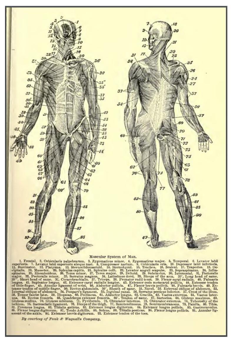
This is a detailed anatomical diagram titled 'Muscular System of Man,' presenting two full-body views of the human musculature: an anterior (front) view on the left and a posterior (back) view on the right. The diagram features numerical labeling (1-93) corresponding to a comprehensive legend at the bottom. The anterior view highlights major muscle groups including the muscles of facial expression, the sternocleidomastoid (13), pectoralis major (31), biceps brachii (35), rectus abdominis (50), and sartorius (67). The posterior view emphasizes the trapezius (17), deltoid (28), latissimus dorsi (34), gluteus maximus (68), and the hamstrings and gastrocnemius (85) of the lower limb. The illustration demonstrates the origin, insertion points, and superficial layering of the human skeletal muscle system. This resource is designed for medical education and provides a systematic overview of musculoskeletal anatomy, useful for identifying specific muscle names and their relative locations within the torso, limbs, and head.
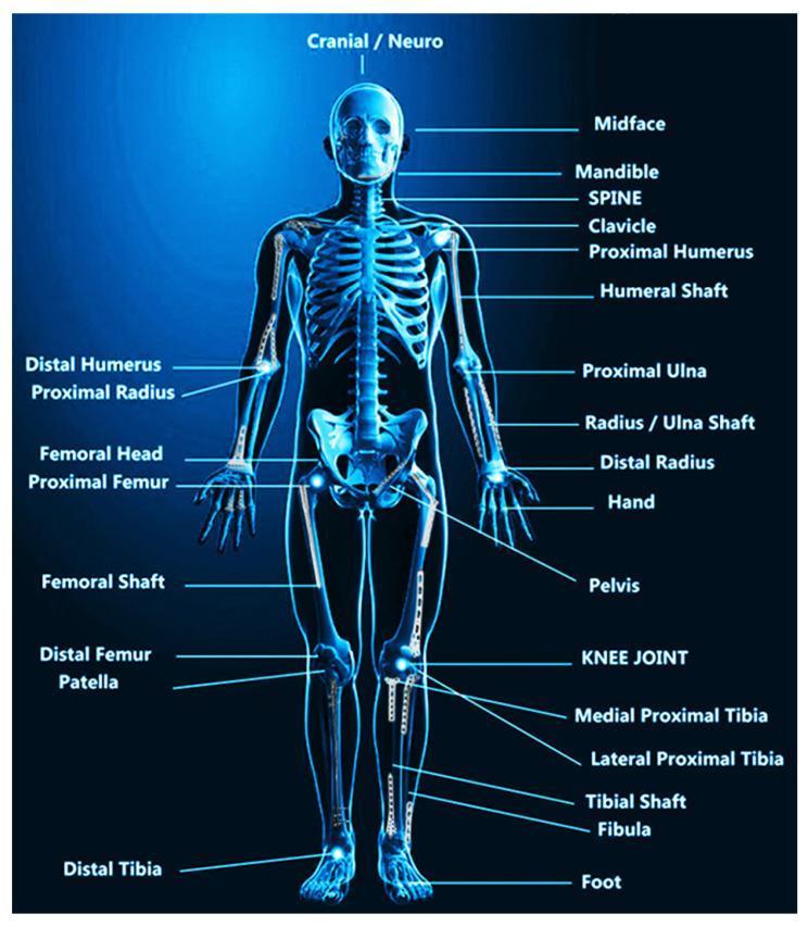
This medical illustration is an anatomical diagram presented as an anterior view of the human skeletal system, styled to resemble an X-ray radiograph. The image provides an educational overview of orthopedic implant locations within the musculoskeletal system. Key anatomical structures labeled include the cranial/neurocranium, midface, mandible, and the spinal column. The upper extremity labels identify the clavicle, proximal and distal humerus, humeral shaft, proximal radius and ulna, and the distal radius. The lower extremity sections highlight the pelvis, femoral head, proximal and distal femur, patella, and knee joint, as well as the medial/lateral proximal tibia, tibial shaft, fibula, and foot. Visually, the diagram overlays clinical imaging of common metallic orthopedic implants—such as bone plates, intramedullary nails, screws, and joint replacements—onto their respective anatomical sites. The primary educational focus is the clinical application and positioning of permanent and temporary fixation devices used in orthopedic surgeries for trauma, joint reconstruction, and managing conditions like osteoporosis.
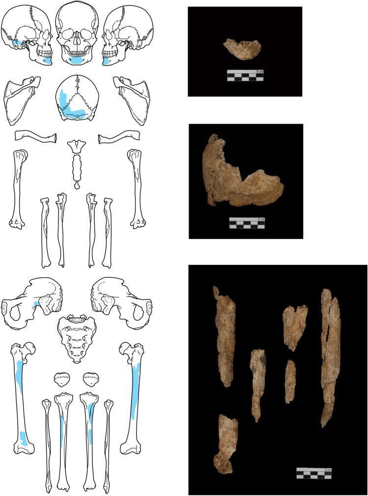
This composite educational image provides an anatomical and forensic overview of excavated human skeletal remains. On the left, an anatomical diagram of a complete human skeleton is presented with specific regions highlighted in blue to indicate recovered fragments. These include sections of the cranium, the mandible, cervical and thoracic vertebrae, parts of the pelvis, and mid-shaft segments of the femur and tibia. On the right, three clinical photographs display the actual archaeological bone fragments against a black background, each accompanied by a 5 cm scale bar. The top photograph shows a partial mandible fragment. The middle photograph depicts a larger, irregular portion of the cranium. The bottom photograph shows multiple longitudinal fragments of cortical bone, consistent with the diaphysis of long bones like the femur or tibia. The bones exhibit a weathered, porous texture and a beige-to-tan coloration indicative of taphonomic changes and mineralization. This visual is designed for physical anthropology and forensic osteology, illustrating the mapping of fragmented remains to the anatomical whole.
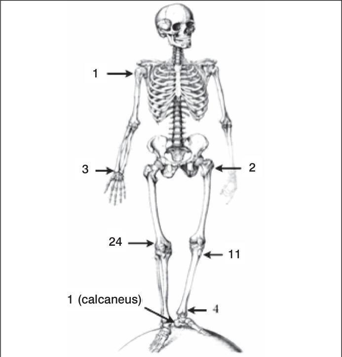
This anatomical diagram presents an anterior view of the human skeletal system, designed as a schematic for mapping orthopedic pathologies such as Giant Cell Tumors (GCT). The illustration features key skeletal components including the skull, axial skeleton (rib cage and vertebrae), pelvis, and appendicular skeleton (upper and lower extremities). Specific anatomical locations are identified with numbered arrows: 1 (proximal humerus/shoulder), 2 (proximal femur/hip), 3 (distal radius/wrist), 24 (distal femur/knee), 11 (proximal tibia), 4 (distal fibula/ankle), and a second label 1 identifying the calcaneus. The diagram serves as a clinical mapping tool to visualize the distribution of bone lesions and helps correlate radiographic classifications, such as Campanacci's bone destruction stages, with specific anatomical sites. It is intended for musculoskeletal oncology education and diagnostic reporting.
axial appendicular skeleton bones labeled diagram
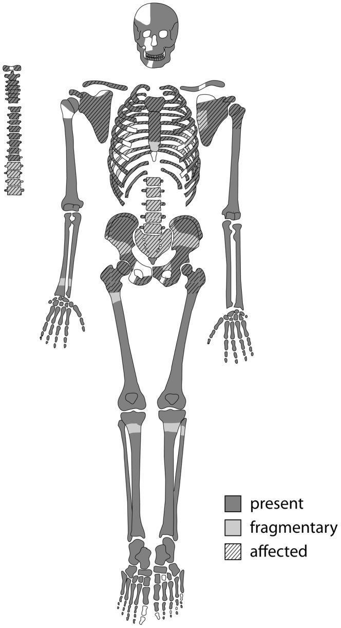
This anatomical diagram is a skeletal inventory and pathology map used in bioarchaeology and paleopathology to document the preservation and disease state of human remains (Skeleton Sk244-8). The graphic uses a standardized human skeletal template with a three-part coding system: dark gray indicates 'present' (full preservation), light gray indicates 'fragmentary' areas, and diagonal hatching denotes bones 'affected' by pathological changes. The map reveals that the axial skeleton—including the sternum, ribs, and most of the vertebral column—is heavily affected by lytic lesions. Both scapulae and the pelvic girdle (innominate bones and sacrum) also show significant involvement with hatching. The appendicular skeleton, specifically the long bones like the humeri, femora, and tibiae, is largely preserved but exhibits localized pathological involvement at the proximal joints. The skull shows a mix of full and fragmentary preservation. This visual summary is essential for illustrating the distribution of systemic skeletal diseases, such as metastatic carcinoma or multiple myeloma, in ancient populations.
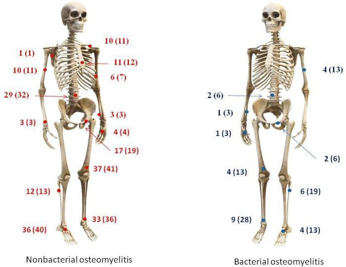
This Comparison Chart consists of two side-by-side anatomical diagrams of the human skeleton, illustrating the distribution and frequency of skeletal foci in nonbacterial osteomyelitis (NBO, left) and bacterial osteomyelitis (BO, right). Each diagram uses colored markers and numerical labels (n values and percentages) to indicate affected anatomical regions. The NBO diagram (red markers) demonstrates a multifocal, widespread distribution across both the axial and appendicular skeleton, with significant involvement of the clavicle, sternum, ribs, spine, femur, tibia, and foot bones. In contrast, the BO diagram (blue markers) displays a more localized or paucifocal pattern, primarily involving the spine, femur, tibia, and fibula, with notable absence of involvement in the clavicle and sternum. This visual comparison highlights key diagnostic differences between the two conditions, emphasizing that multifocality and involvement of the axial skeleton (beyond the spine) are highly suggestive of a nonbacterial etiology. The educational focus is on the clinical differentiation of pediatric bone infections and inflammatory disorders through skeletal mapping.
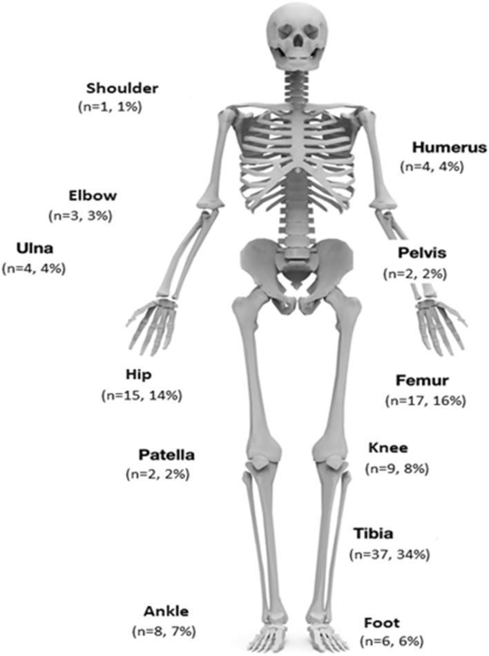
This infographic presents an anatomical diagram of the human skeleton used as a data visualization tool to map the distribution of orthopedic infections across various skeletal sites. The diagram provides quantitative data for 107 cases, labeling specific bones and joints with the number of patients (n) and the corresponding percentage of the total study population. Labeled anatomical regions include the upper extremity (shoulder, humerus, elbow, and ulna), the axial/pelvic region (pelvis), and the lower extremity (hip, femur, knee, patella, tibia, ankle, and foot). The visualization highlights the tibia as the most frequent site of infection (n=37, 34%), followed by the femur (n=17, 16%) and hip (n=15, 14%). This clinical illustration is designed for orthopedic and infectious disease education, effectively demonstrating the anatomical prevalence of conditions such as fracture-related infection (FRI), chronic osteomyelitis (COM), and prosthetic joint infection (PJI) within a clinical cohort.
long bone anatomy diaphysis epiphysis periosteum compact spongy bone
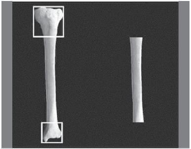
This clinical photograph displays a comparative view of long bone specimen preparation for orthopedic research. On the left, a complete tibia is shown with the proximal and distal epiphyses highlighted by white squares, demonstrating the application of Heim's square to identify the epiphysis-diaphysis transition. On the right, the resulting isolated diaphyseal segment is shown following osteotomy at those precise levels. The specimens exhibit a smooth, off-white surface texture, indicating thorough removal of soft tissue and the periosteum. The image illustrates the standardized anatomical methodology used to obtain uniform diaphyseal bone segments for clinical research, such as biomechanical testing or ultrasonometric analysis of fracture fixation methods. The focus is on the anatomical landmarks and the geometric precision required to isolate the shaft while maintaining consistency across experimental samples.
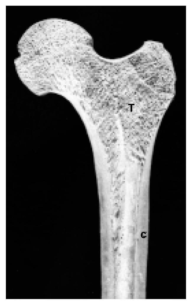
This diagnostic image is a longitudinal section of the proximal femur, illustrating the macrostructure of human long bones. The anatomical region shown includes the femoral head, neck, and the superior portion of the femoral shaft. Two distinct bone types are labeled for educational comparison. The area labeled 'C' represents the cortical bone (compact bone) forming the thick, dense outer walls of the diaphysis. It is characterized by a solid, uniform radiopaque appearance with high density and structural rigidity. The area labeled 'T' identifies the cancellous bone (spongy or trabecular bone) concentrated within the epiphysis and metaphysis. This region displays a characteristic porous, meshwork-like organization consisting of thin plates and interconnected trabeculae. The visual highlights the transition between the load-bearing cortical shell and the internal honeycomb-like support system of the femur, providing an anatomical basis for understanding bone physiology and structural integrity in orthopedics and endocrinology.
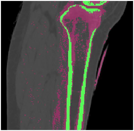
This diagnostic image is a color-coded 2D cross-section of a human leg, derived from CT imaging of the proximal tibia and fibula. The visualization uses threshold-based segmentation to distinguish between different bone compositions for orthopedic modeling. The cortical bone (compact bone) is highlighted in bright green, forming a thick, dense outer shell along the diaphysis and maintaining structural integrity. The cancellous bone (trabecular or spongy bone) is represented in rose pink, primarily concentrated within the proximal epiphysis and metaphysis. This distribution highlights the anatomical transition from the high-density load-bearing cortical shaft to the internal network of cancellous bone at the joints, which facilitates force distribution. This image serves as a foundational step for biomechanical finite element analysis, such as simulating tibial plateau fractures or assessing the impacts of osteoporosis on bone density and surgical fixation stability.
types of cartilage hyaline elastic fibrocartilage histology
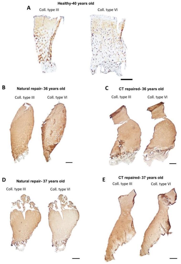
This diagnostic image set displays immunohistochemistry (IHC) staining of human articular cartilage core biopsies, comparing healthy tissue (A) with naturally repaired (B, D) and cell therapy (CT) repaired cartilage (C, E). The panels evaluate the spatial distribution of collagen type III and collagen type VI. In healthy cartilage (A), collagen type III is localized in the interterritorial matrix, whereas collagen type VI shows specific pericellular staining surrounding chondrocytes. In samples B and C (hyaline-like repair), these distinct localization patterns are partially preserved. In contrast, samples D and E (fibrocartilage repair) demonstrate a loss of specific regionalization, characterized by a more diffuse, homogenous staining pattern of both collagen types throughout the dense matrix. The images highlight differences in matrix organization and quality between hyaline and fibrocartilaginous repair tissues, serving as a markers for tissue regeneration success. Scale bars represent 500 µm.
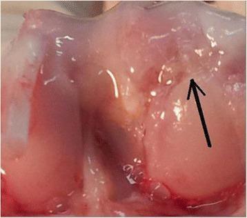
This clinical photograph shows a macroscopic view of an articular joint surface, specifically focusing on a focal cartilage defect undergoing repair. The image highlights a specific lesion (indicated by a black arrow) characterized by significant surface irregularities. The repairing tissue within the defect exhibits a distinct purple-whitish color and a textured, uneven morphology compared to the smooth, glistening appearance of the surrounding healthy hyaline cartilage. This visual illustrates the outcome of a microfracture (mfx) surgical procedure, demonstrating the formation of fibrocartilage-like repair tissue which often lacks the structural regularity and integration seen in higher-quality hyaline-like repair. The image serves as a clinical reference for orthopedic evaluation of cartilage regeneration, specifically showcasing the characteristic irregular surface of early or suboptimal healing in a microfracture-only treatment group.
Introduction to the Skeletal System
1. Overview
2. Functions of the Skeletal System
| Function | Detail |
|---|---|
| Structural support | Forms the body's load-bearing framework |
| Protection | Shields vital organs (e.g., skull protects brain, rib cage protects heart and lungs) |
| Mineral reservoir | Stores calcium and phosphorus; maintains serum homeostasis and acid-base balance |
| Movement | Acts as levers on which muscles act |
| Hematopoiesis | Contains bone marrow that produces blood cells |
3. Divisions of the Skeleton
Axial Skeleton (80 bones)
- Skull (cranium)
- Vertebral column
- Ribs
- Sternum
Appendicular Skeleton (126 bones)
- Bones of the upper limbs
- Bones of the lower limbs
- Shoulder girdle (clavicle, scapula)
- Pelvic girdle
The 6 auditory ossicles (malleus, incus, stapes - in each ear) bring the total to 206.
4. Classification of Bones by Shape
| Type | Description | Example |
|---|---|---|
| Long bones | Tubular; longer than wide | Humerus, femur, metacarpals, phalanges |
| Short bones | Cuboidal; roughly equal dimensions | Carpal and tarsal bones |
| Flat bones | Two compact plates with spongy bone between | Skull, scapula |
| Irregular bones | Complex shapes that don't fit other categories | Vertebrae, facial bones, hyoid |
| Sesamoid bones | Round/oval; develop within tendons | Patella (largest), thumb and big toe tendons |
5. Bone Tissue - Compact vs. Spongy
-
Compact (cortical) bone - Dense outer shell forming ~80% of skeletal mass. The diaphysis (shaft) of long bones is primarily compact bone. Organized into cylindrical units called Haversian systems (osteons), each with concentric lamellae around a central Haversian canal carrying vessels and nerves.
-
Spongy (cancellous/trabecular) bone - Honeycomb-like meshwork of trabeculae that fill the epiphyses and metaphyses. Highly vascular and the major site of hematopoiesis. Trabeculae align along lines of mechanical stress.
Gross Anatomy of a Long Bone
| Region | Description |
|---|---|
| Diaphysis | Tubular shaft; thick cortical bone surrounding the medullary cavity |
| Epiphysis | Rounded ends; mostly spongy bone covered by a thin cortical shell |
| Metaphysis | Cone-shaped transition zone connecting diaphysis and epiphysis |
| Growth plate (physis) | Cartilaginous interface between metaphysis and epiphysis (in growing bone) |
| Periosteum | Fibrous membrane covering all bone surfaces except at joints; capable of forming new bone |
| Medullary cavity | Central space containing bone marrow |
6. Bone Cells
| Cell | Origin | Function |
|---|---|---|
| Osteoblasts | Mesenchymal stem cells | Synthesize bone matrix (osteoid); produce osteoprotegerin |
| Osteocytes | Derived from osteoblasts | Enclosed in lacunae; main mechanosensing cells; regulate remodeling via sclerostin |
| Osteoclasts | Hematopoietic lineage (macrophages) | Resorb bone; activated by RANKL signaling |
7. Bone Composition
- Collagenous matrix (osteoid) - mainly Type I collagen
- Hydroxyapatite crystals - calcium phosphate mineral providing rigidity
- Cellular components - osteoblasts, osteocytes, osteoclasts
- Blood vessels and nerves - via Haversian and Volkmann's canals
8. Cartilage
| Type | Fiber Content | Location |
|---|---|---|
| Hyaline | Moderate collagen | Articular surfaces, costal cartilages, nose, trachea |
| Elastic | Collagen + abundant elastic fibers | External ear, epiglottis |
| Fibrocartilage | Dense collagen, few cells | Intervertebral discs, pubic symphysis, menisci |
9. Bone Development (Ossification)
-
Intramembranous ossification - Mesenchymal cells differentiate directly into osteoblasts without a cartilage precursor. Produces flat bones of the skull, mandible, and clavicle.
-
Endochondral ossification - A cartilage model forms first, then is replaced by bone. This is how most bones form, including all long bones. (Histology: A Text and Atlas; Robbins & Kumar Basic Pathology)
10. Vascular and Nerve Supply
- A nutrient artery (usually one per bone) enters the internal cavity and supplies the marrow, spongy bone, and inner compact bone.
- The periosteum receives branches from adjacent vessels supplying the outer compact bone. A bone stripped of periosteum will not survive.
- Bone itself has few sensory fibers, but the periosteum is densely innervated and highly sensitive to injury - explaining why periosteal injuries are so painful.