"""
Comprehensive Study Guide PDF: Physiology of Hearing & Vision
Source: Guyton and Hall Textbook of Medical Physiology
"""

import requests
import os
from io import BytesIO
from PIL import Image as PILImage

from reportlab.lib.pagesizes import A4
from reportlab.lib import colors
from reportlab.lib.styles import getSampleStyleSheet, ParagraphStyle
from reportlab.lib.units import mm, cm, inch
from reportlab.lib.enums import TA_CENTER, TA_LEFT, TA_JUSTIFY
from reportlab.platypus import (
    SimpleDocTemplate, Paragraph, Spacer, Table, TableStyle,
    Image, PageBreak, HRFlowable, KeepTogether
)
from reportlab.platypus.tableofcontents import TableOfContents
from reportlab.pdfgen import canvas
from reportlab.lib.colors import HexColor

OUTPUT = "/home/daytona/workspace/hearing-vision-guide/Hearing_Vision_Study_Guide.pdf"

# ── Colour palette ─────────────────────────────────────────────────────────────
NAVY      = HexColor("#1a2e5a")
TEAL      = HexColor("#0a7e8c")
LIGHT_BG  = HexColor("#eaf4f6")
ACCENT    = HexColor("#e8f0fe")
GOLD      = HexColor("#c0820a")
RED_DARK  = HexColor("#8b1a1a")
GREEN_DK  = HexColor("#1a5c2a")
GREY_LT   = HexColor("#f5f5f5")
GREY_MID  = HexColor("#d0d0d0")
WHITE     = colors.white
BLACK     = colors.black

# ── Image URLs ─────────────────────────────────────────────────────────────────
IMAGES = {
    "ear_anatomy":    "https://cdn.orris.care/cdss_images/50888ba37b5638f32512d96c895e2490b7663d381efdd9e39643353336a00bfc.png",
    "traveling_wave": "https://cdn.orris.care/cdss_images/706f51aec2d69fe5272c1e9ac25f426da88d4e18ea60d98455476af1af90662c.png",
    "eye_retina":     "https://cdn.orris.care/cdss_images/c0fc505230afc6a54194c0a61311c30a797cb09f8af52077a22c6a1b9ed090ce.png",
    "rod_cone":       "https://cdn.orris.care/cdss_images/1a3e831d77deb9e2e17092b18f0d4c400ad17a3ae207301f1f503a3d6bf50bbd.png",
    "visual_pathway": "https://cdn.orris.care/cdss_images/e3eb6b81926026f5ebb54992e4911d857423f33760d38bfe6fa89f19b5d3e2b7.png",
}

IMG_CACHE = {}

def download_image(key, url):
    """Download and cache image, return ReportLab Image object or None."""
    if key in IMG_CACHE:
        return IMG_CACHE[key]
    try:
        r = requests.get(url, timeout=15)
        r.raise_for_status()
        img_data = BytesIO(r.content)
        pil = PILImage.open(img_data)
        w, h = pil.size
        img_data.seek(0)
        IMG_CACHE[key] = (img_data, w, h)
        print(f"  Downloaded: {key} ({w}x{h})")
        return IMG_CACHE[key]
    except Exception as e:
        print(f"  WARN: Could not download {key}: {e}")
        return None

def make_image(key, url, max_width, max_height=None):
    """Return a ReportLab Image scaled to fit max_width."""
    result = download_image(key, url)
    if result is None:
        return Spacer(1, 5*mm)
    img_data, w, h = result
    aspect = h / w
    img_w = min(max_width, w)
    img_h = img_w * aspect
    if max_height and img_h > max_height:
        img_h = max_height
        img_w = img_h / aspect
    img_data.seek(0)
    return Image(img_data, width=img_w, height=img_h)


# ── Styles ──────────────────────────────────────────────────────────────────────
def build_styles():
    base = getSampleStyleSheet()

    styles = {}

    styles["cover_title"] = ParagraphStyle(
        "cover_title", parent=base["Title"],
        fontSize=28, textColor=WHITE, alignment=TA_CENTER,
        spaceAfter=6, leading=34, fontName="Helvetica-Bold"
    )
    styles["cover_sub"] = ParagraphStyle(
        "cover_sub", parent=base["Normal"],
        fontSize=14, textColor=HexColor("#cce8f0"), alignment=TA_CENTER,
        spaceAfter=4, leading=18, fontName="Helvetica"
    )
    styles["cover_note"] = ParagraphStyle(
        "cover_note", parent=base["Normal"],
        fontSize=10, textColor=HexColor("#aad4e0"), alignment=TA_CENTER,
        spaceAfter=4, leading=14, fontName="Helvetica-Oblique"
    )
    styles["part_header"] = ParagraphStyle(
        "part_header", parent=base["Heading1"],
        fontSize=22, textColor=WHITE, alignment=TA_CENTER,
        spaceAfter=8, spaceBefore=0, leading=28, fontName="Helvetica-Bold"
    )
    styles["h1"] = ParagraphStyle(
        "h1", parent=base["Heading1"],
        fontSize=16, textColor=NAVY, spaceBefore=14, spaceAfter=6,
        leading=20, fontName="Helvetica-Bold", borderPad=4,
        borderColor=TEAL, borderWidth=0
    )
    styles["h2"] = ParagraphStyle(
        "h2", parent=base["Heading2"],
        fontSize=13, textColor=TEAL, spaceBefore=10, spaceAfter=4,
        leading=17, fontName="Helvetica-Bold"
    )
    styles["h3"] = ParagraphStyle(
        "h3", parent=base["Heading3"],
        fontSize=11, textColor=NAVY, spaceBefore=8, spaceAfter=3,
        leading=15, fontName="Helvetica-Bold"
    )
    styles["body"] = ParagraphStyle(
        "body", parent=base["Normal"],
        fontSize=10, textColor=BLACK, spaceBefore=3, spaceAfter=3,
        leading=15, fontName="Helvetica", alignment=TA_JUSTIFY
    )
    styles["body_b"] = ParagraphStyle(
        "body_b", parent=base["Normal"],
        fontSize=10, textColor=BLACK, spaceBefore=2, spaceAfter=2,
        leading=15, fontName="Helvetica-Bold"
    )
    styles["bullet"] = ParagraphStyle(
        "bullet", parent=base["Normal"],
        fontSize=10, textColor=BLACK, spaceBefore=2, spaceAfter=2,
        leading=14, fontName="Helvetica", leftIndent=14, bulletIndent=0
    )
    styles["caption"] = ParagraphStyle(
        "caption", parent=base["Normal"],
        fontSize=8.5, textColor=HexColor("#444444"), alignment=TA_CENTER,
        spaceAfter=6, leading=12, fontName="Helvetica-Oblique"
    )
    styles["box_title"] = ParagraphStyle(
        "box_title", parent=base["Normal"],
        fontSize=10.5, textColor=NAVY, spaceBefore=0, spaceAfter=3,
        leading=14, fontName="Helvetica-Bold"
    )
    styles["box_body"] = ParagraphStyle(
        "box_body", parent=base["Normal"],
        fontSize=9.5, textColor=BLACK, spaceBefore=2, spaceAfter=2,
        leading=13, fontName="Helvetica"
    )
    styles["key_fact"] = ParagraphStyle(
        "key_fact", parent=base["Normal"],
        fontSize=10, textColor=RED_DARK, spaceBefore=4, spaceAfter=4,
        leading=14, fontName="Helvetica-Bold"
    )
    styles["footer"] = ParagraphStyle(
        "footer", parent=base["Normal"],
        fontSize=8, textColor=HexColor("#888888"), alignment=TA_CENTER,
        fontName="Helvetica-Oblique"
    )

    return styles

S = build_styles()

# ── Helper builders ─────────────────────────────────────────────────────────────

def section_divider(title, color=TEAL):
    """A full-width coloured section banner."""
    data = [[Paragraph(title, ParagraphStyle(
        "sdiv", fontSize=13, textColor=WHITE, fontName="Helvetica-Bold",
        alignment=TA_CENTER, leading=18
    ))]]
    t = Table(data, colWidths=[170*mm])
    t.setStyle(TableStyle([
        ("BACKGROUND", (0,0), (-1,-1), color),
        ("TOPPADDING",    (0,0), (-1,-1), 6),
        ("BOTTOMPADDING", (0,0), (-1,-1), 6),
        ("LEFTPADDING",   (0,0), (-1,-1), 8),
        ("RIGHTPADDING",  (0,0), (-1,-1), 8),
    ]))
    return t

def info_box(title, lines, bg=ACCENT, title_color=NAVY):
    """Styled box for key points / clinical notes."""
    content = [Paragraph(title, ParagraphStyle(
        "ib_t", fontSize=10.5, textColor=title_color, fontName="Helvetica-Bold", leading=14
    ))]
    for ln in lines:
        content.append(Paragraph(f"• {ln}", ParagraphStyle(
            "ib_b", fontSize=9.5, textColor=BLACK, fontName="Helvetica", leading=13, leftIndent=8
        )))
    data = [[content]]
    t = Table(data, colWidths=[168*mm])
    t.setStyle(TableStyle([
        ("BACKGROUND", (0,0), (-1,-1), bg),
        ("BOX",        (0,0), (-1,-1), 1, HexColor("#b0c8d8")),
        ("TOPPADDING",    (0,0), (-1,-1), 8),
        ("BOTTOMPADDING", (0,0), (-1,-1), 8),
        ("LEFTPADDING",   (0,0), (-1,-1), 10),
        ("RIGHTPADDING",  (0,0), (-1,-1), 10),
        ("VALIGN",     (0,0), (-1,-1), "TOP"),
    ]))
    return t

def styled_table(headers, rows, col_widths=None):
    """Two-tone striped data table."""
    data = [headers] + rows
    n_cols = len(headers)
    if col_widths is None:
        col_widths = [170*mm / n_cols] * n_cols

    header_style = ParagraphStyle("th", fontSize=9.5, textColor=WHITE,
                                   fontName="Helvetica-Bold", leading=13, alignment=TA_CENTER)
    cell_style   = ParagraphStyle("td", fontSize=9,   textColor=BLACK,
                                   fontName="Helvetica", leading=12, alignment=TA_LEFT)

    fmt_data = []
    for i, row in enumerate(data):
        fmt_row = []
        for cell in row:
            style = header_style if i == 0 else cell_style
            fmt_row.append(Paragraph(str(cell), style))
        fmt_data.append(fmt_row)

    t = Table(fmt_data, colWidths=col_widths, repeatRows=1)
    ts = [
        ("BACKGROUND", (0,0), (-1,0), NAVY),
        ("ROWBACKGROUNDS", (0,1), (-1,-1), [WHITE, GREY_LT]),
        ("BOX",       (0,0), (-1,-1), 0.5, GREY_MID),
        ("INNERGRID", (0,0), (-1,-1), 0.3, GREY_MID),
        ("TOPPADDING",    (0,0), (-1,-1), 5),
        ("BOTTOMPADDING", (0,0), (-1,-1), 5),
        ("LEFTPADDING",   (0,0), (-1,-1), 6),
        ("RIGHTPADDING",  (0,0), (-1,-1), 6),
        ("VALIGN",    (0,0), (-1,-1), "MIDDLE"),
    ]
    t.setStyle(TableStyle(ts))
    return t

def h1(text): return Paragraph(text, S["h1"])
def h2(text): return Paragraph(text, S["h2"])
def h3(text): return Paragraph(text, S["h3"])
def p(text):  return Paragraph(text, S["body"])
def pb(text): return Paragraph(text, S["body_b"])
def kf(text): return Paragraph(f"★ KEY FACT: {text}", S["key_fact"])
def sp(n=1):  return Spacer(1, n*4*mm)
def hr():     return HRFlowable(width="100%", thickness=0.5, color=GREY_MID, spaceAfter=3, spaceBefore=3)
def cap(text): return Paragraph(text, S["caption"])
def bul(items):
    return [Paragraph(f"• {i}", S["bullet"]) for i in items]


# ═══════════════════════════════════════════════════════════════════════════════
#  PAGE LAYOUT / TEMPLATES
# ═══════════════════════════════════════════════════════════════════════════════

class MyDocTemplate(SimpleDocTemplate):
    def __init__(self, filename, **kw):
        super().__init__(filename, **kw)
        self.page_num = 0

    def handle_pageBegin(self):
        self.page_num += 1
        super().handle_pageBegin()

def on_page(canvas, doc):
    """Header/footer on every page except cover."""
    if doc.page <= 1:
        return
    canvas.saveState()
    W, H = A4
    # Top band
    canvas.setFillColor(NAVY)
    canvas.rect(0, H - 14*mm, W, 14*mm, fill=1, stroke=0)
    canvas.setFont("Helvetica-Bold", 8)
    canvas.setFillColor(WHITE)
    canvas.drawString(15*mm, H - 9*mm, "PHYSIOLOGY OF HEARING & VISION")
    canvas.drawRightString(W - 15*mm, H - 9*mm, "Guyton and Hall · Medical Physiology")
    # Bottom band
    canvas.setFillColor(NAVY)
    canvas.rect(0, 0, W, 10*mm, fill=1, stroke=0)
    canvas.setFont("Helvetica", 8)
    canvas.setFillColor(WHITE)
    canvas.drawCentredString(W/2, 3.5*mm, f"Page {doc.page}")
    canvas.restoreState()


# ═══════════════════════════════════════════════════════════════════════════════
#  CONTENT BUILDERS
# ═══════════════════════════════════════════════════════════════════════════════

def cover_page():
    """Full navy cover with title block."""
    W, H = A4
    elems = []

    # Big navy background table
    cover_block = [
        [Paragraph("COMPREHENSIVE STUDY GUIDE", ParagraphStyle(
            "ct", fontSize=11, textColor=HexColor("#aad4e0"), alignment=TA_CENTER,
            fontName="Helvetica", leading=16, spaceAfter=6
        ))],
        [Paragraph("Physiology of Hearing &amp; Vision", ParagraphStyle(
            "ctm", fontSize=30, textColor=WHITE, alignment=TA_CENTER,
            fontName="Helvetica-Bold", leading=36, spaceAfter=8
        ))],
        [Paragraph("Outer Ear · Middle Ear · Inner Ear<br/>Functional Anatomy of the Eye<br/>Retina · Visual Pathways · Visual Cortex", ParagraphStyle(
            "ctsub", fontSize=14, textColor=HexColor("#cce8f0"), alignment=TA_CENTER,
            fontName="Helvetica", leading=22, spaceAfter=20
        ))],
        [Spacer(1, 12*mm)],
        [HRFlowable(width="80%", thickness=1, color=HexColor("#4488aa"), spaceAfter=10, spaceBefore=0)],
        [Paragraph("Source: Guyton and Hall Textbook of Medical Physiology", ParagraphStyle(
            "csrc", fontSize=11, textColor=HexColor("#88c8d8"), alignment=TA_CENTER,
            fontName="Helvetica-Oblique", leading=16
        ))],
        [Paragraph("ISBN: 9780443111013", ParagraphStyle(
            "cisbn", fontSize=10, textColor=HexColor("#6699aa"), alignment=TA_CENTER,
            fontName="Helvetica", leading=14
        ))],
        [Spacer(1, 8*mm)],
        [Paragraph("Chapters 50 – 53  ·  Complete Notes with Diagrams  ·  Exam Prep Edition", ParagraphStyle(
            "cch", fontSize=10, textColor=HexColor("#aad4e0"), alignment=TA_CENTER,
            fontName="Helvetica-Oblique", leading=14
        ))],
    ]

    t = Table(cover_block, colWidths=[170*mm])
    t.setStyle(TableStyle([
        ("BACKGROUND",    (0,0), (-1,-1), NAVY),
        ("TOPPADDING",    (0,0), (-1,-1), 6),
        ("BOTTOMPADDING", (0,0), (-1,-1), 6),
        ("LEFTPADDING",   (0,0), (-1,-1), 20),
        ("RIGHTPADDING",  (0,0), (-1,-1), 20),
        ("ALIGN",         (0,0), (-1,-1), "CENTER"),
    ]))

    elems.append(Spacer(1, 30*mm))
    elems.append(t)
    elems.append(PageBreak())
    return elems


def toc_section():
    elems = []
    elems.append(sp(2))
    elems.append(section_divider("TABLE OF CONTENTS", NAVY))
    elems.append(sp(1))

    toc_items = [
        ("PART I: PHYSIOLOGY OF HEARING", ""),
        ("  1.  The Outer Ear", ""),
        ("  2.  The Middle Ear – Ossicular System & Impedance Matching", ""),
        ("  3.  The Inner Ear – Cochlea & Frequency Analysis", ""),
        ("  4.  Organ of Corti & Transduction", ""),
        ("  5.  Central Auditory Pathways", ""),
        ("  6.  Sound Localization", ""),
        ("  7.  Auditory Cortex", ""),
        ("PART II: PHYSIOLOGY OF VISION", ""),
        ("  8.  Optics of the Eye & Accommodation", ""),
        ("  9.  Refractive Errors", ""),
        ("  10. Retina – Functional Anatomy", ""),
        ("  11. Photoreceptors: Rods & Cones", ""),
        ("  12. Phototransduction", ""),
        ("  13. Color Vision", ""),
        ("  14. Retinal Neural Processing", ""),
        ("  15. Central Visual Pathways – Retina to Cortex", ""),
        ("  16. Lateral Geniculate Nucleus", ""),
        ("  17. Primary Visual Cortex (V1)", ""),
        ("  18. Dorsal & Ventral Visual Streams", ""),
        ("  19. Pupillary Reflexes", ""),
        ("QUICK REFERENCE TABLES & CLINICAL CORRELATIONS", ""),
    ]

    for title, page in toc_items:
        is_part = title.startswith("PART") or title.startswith("QUICK")
        style = ParagraphStyle(
            "toc_part" if is_part else "toc_item",
            fontSize=11 if is_part else 9.5,
            textColor=NAVY if is_part else BLACK,
            fontName="Helvetica-Bold" if is_part else "Helvetica",
            leading=17 if is_part else 14,
            spaceBefore=6 if is_part else 2,
            leftIndent=0 if is_part else 10
        )
        elems.append(Paragraph(title, style))

    elems.append(PageBreak())
    return elems


# ─── PART I: HEARING ──────────────────────────────────────────────────────────

def part1_hearing(page_w):
    elems = []

    # Part banner
    data = [[Paragraph("PART I: PHYSIOLOGY OF HEARING", ParagraphStyle(
        "ph", fontSize=20, textColor=WHITE, fontName="Helvetica-Bold",
        alignment=TA_CENTER, leading=26
    ))]]
    t = Table(data, colWidths=[170*mm])
    t.setStyle(TableStyle([
        ("BACKGROUND", (0,0), (-1,-1), NAVY),
        ("TOPPADDING",    (0,0), (-1,-1), 14),
        ("BOTTOMPADDING", (0,0), (-1,-1), 14),
    ]))
    elems.append(sp(1))
    elems.append(t)
    elems.append(sp(2))

    # Ear anatomy diagram
    img = make_image("ear_anatomy", IMAGES["ear_anatomy"], page_w * 0.92, 110*mm)
    elems.append(img)
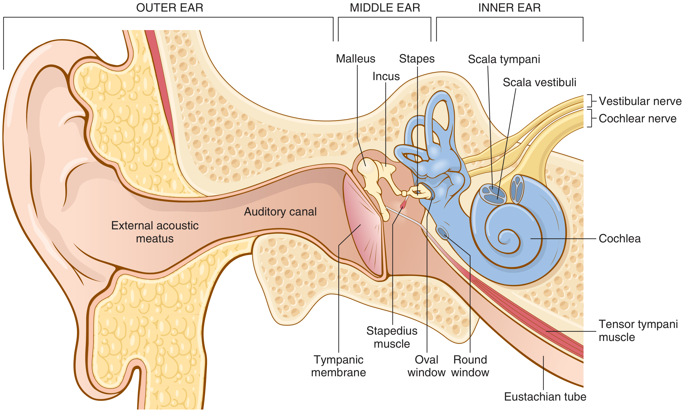
    elems.append(cap("Fig. 53.1 — The outer ear, tympanic membrane, and ossicular system of the middle ear and inner ear. (Guyton & Hall)"))
    elems.append(sp(1))

    # Overview
    elems.append(p("Sound is conducted through three anatomical regions: the <b>outer ear</b> (sound collection and direction), "
                   "the <b>middle ear</b> (mechanical amplification and impedance matching), and the <b>inner ear/cochlea</b> "
                   "(frequency analysis and transduction into nerve impulses)."))
    elems.append(sp(1))

    # ── 1. OUTER EAR ─────────────────────────────────────────────────────────
    elems.append(section_divider("1. THE OUTER EAR"))
    elems.append(sp(1))

    elems.append(h2("Components"))
    elems += bul([
        "<b>Pinna (auricle):</b> Cartilaginous funnel that collects sound waves and directs them into the external auditory canal. "
        "Its irregular shape modifies the frequency spectrum of incoming sound depending on direction, enabling "
        "discrimination of sounds from in front vs. behind and above vs. below.",
        "<b>External auditory meatus (canal):</b> ~2.5 cm long, curved tube from pinna to tympanic membrane. "
        "Hairs and cerumen (earwax) protect the delicate tympanic membrane.",
        "<b>Tympanic membrane (eardrum):</b> Cone-shaped, tense membrane that vibrates with sound waves. "
        "The handle of the malleus is attached to its center. Kept under constant tension by the <i>tensor tympani</i> muscle "
        "so that vibrations on any portion are transmitted to the ossicles."
    ])
    elems.append(sp(1))
    elems.append(info_box("Key Point: Pinna Function",
        ["The pinna cannot distinguish front vs. back or up vs. down by time-lag alone — it does so by "
         "selectively filtering the frequency content of sounds arriving from different directions."],
        bg=LIGHT_BG))
    elems.append(sp(1))

    # ── 2. MIDDLE EAR ────────────────────────────────────────────────────────
    elems.append(section_divider("2. THE MIDDLE EAR"))
    elems.append(sp(1))

    elems.append(h2("The Ossicular System"))
    elems.append(p("Three tiny bones form a mechanical lever that transmits tympanic membrane vibrations to the oval window of the cochlea:"))
    elems.append(sp(1))

    ossicle_table = styled_table(
        ["Ossicle", "Position in Chain", "Key Attachment"],
        [
            ["Malleus (hammer)", "Lateral — attached to tympanic membrane", "Handle (manubrium) fused to center of eardrum; head articulates with incus"],
            ["Incus (anvil)",    "Middle — bridge bone",                    "Body with malleus; long process with stapes"],
            ["Stapes (stirrup)", "Medial — innermost ossicle",              "Footplate sits in oval window of cochlea"],
        ],
        col_widths=[40*mm, 65*mm, 65*mm]
    )
    elems.append(ossicle_table)
    elems.append(sp(1))

    elems.append(h2("Impedance Matching — The Critical Function"))
    elems.append(p("Fluid (perilymph) has far greater inertia than air. The ossicular system converts low-force, "
                   "large-amplitude sound waves in air to high-force, small-amplitude vibrations in cochlear fluid."))
    elems.append(sp(0.5))

    impedance_data = styled_table(
        ["Parameter", "Value / Effect"],
        [
            ["Tympanic membrane surface area", "~55 mm²"],
            ["Stapes footplate surface area", "~3.2 mm²"],
            ["Area ratio", "~17:1"],
            ["Lever force amplification", "~1.3×"],
            ["Total force amplification on cochlear fluid", "~22× (17 × 1.3)"],
            ["Efficiency (300–3000 Hz)", "50–75% of perfect impedance match"],
            ["Without ossicles (direct air conduction)", "15–20 dB less sensitive"],
        ],
        col_widths=[90*mm, 80*mm]
    )
    elems.append(impedance_data)
    elems.append(sp(0.5))
    elems.append(kf("The ossicular lever reduces amplitude but increases force ~22-fold, matching the acoustic impedance of air to fluid."))
    elems.append(sp(1))

    elems.append(h2("Attenuation Reflex (Acoustic Reflex / Sound Protection)"))
    elems.append(p("Loud sounds (>70 dB) reflexively contract two muscles after a latency of 40–60 ms:"))
    elems += bul([
        "<b>Tensor tympani muscle:</b> Pulls malleus inward, increasing tension on the tympanic membrane",
        "<b>Stapedius muscle:</b> Pulls stapes posteriorly, reducing inward excursion of the oval window",
        "Net effect: Reduces transmission of <b>low-frequency sounds</b> (below ~1000 Hz)",
        "Protects cochlea from sustained loud noise — <i>not</i> from sudden impulse sounds (latency too long)",
        "Also reduces loudness of the person's own voice (efferent feedback)"
    ])
    elems.append(sp(1))

    elems.append(h2("Eustachian (Pharyngotympanic) Tube"))
    elems += bul([
        "Connects middle ear to nasopharynx; normally collapsed, opens during swallowing/yawning",
        "Equalizes air pressure between middle ear and atmosphere",
        "Blockage (e.g., upper respiratory infection) → pressure difference → dampened ossicular movement → conductive hearing loss"
    ])
    elems.append(sp(1))
    elems.append(PageBreak())

    # ── 3. INNER EAR ─────────────────────────────────────────────────────────
    elems.append(section_divider("3. THE INNER EAR (COCHLEA)"))
    elems.append(sp(1))

    elems.append(h2("Cochlear Structure"))
    elems.append(p("The cochlea is a fluid-filled bony spiral of 2.5 turns, divided into three fluid-filled compartments:"))
    elems.append(sp(0.5))

    cochlea_table = styled_table(
        ["Compartment", "Fluid", "Location", "Boundaries"],
        [
            ["Scala vestibuli", "Perilymph (low K⁺, high Na⁺)", "Upper",  "Reissner's membrane (below)"],
            ["Scala media (cochlear duct)", "Endolymph (high K⁺, low Na⁺)", "Middle", "Reissner's (above) & basilar membrane (below)"],
            ["Scala tympani", "Perilymph", "Lower", "Basilar membrane (above); round window at base"],
        ],
        col_widths=[42*mm, 45*mm, 22*mm, 61*mm]
    )
    elems.append(cochlea_table)
    elems.append(sp(0.5))
    elems += bul([
        "Scala vestibuli and scala tympani communicate at the <b>helicotrema</b> (apex of cochlea)",
        "Oval window: stapes footplate transmits vibrations → scala vestibuli",
        "Round window: compensatory membrane at base of scala tympani that bulges outward when oval window moves inward"
    ])
    elems.append(sp(1))

    elems.append(h2("The Basilar Membrane — Frequency (Tonotopic) Map"))
    elems.append(p("The basilar membrane runs the length of the cochlea (~35 mm) and varies in its mechanical properties:"))
    elems.append(sp(0.5))

    basilar_table = styled_table(
        ["Location", "Basilar Fiber Width", "Stiffness", "Resonant Frequency"],
        [
            ["Base (near oval window)", "Narrow (~0.04 mm)", "Stiff", "High (~20,000 Hz)"],
            ["Midpoint",               "Intermediate",       "Intermediate", "~1,000–2,000 Hz"],
            ["Apex (helicotrema)",      "Wide (~0.5 mm)",    "Floppy", "Low (~20 Hz)"],
        ],
        col_widths=[50*mm, 40*mm, 35*mm, 45*mm]
    )
    elems.append(basilar_table)
    elems.append(sp(0.5))
    elems.append(info_box("Tonotopic Principle",
        ["Each frequency of sound causes maximal vibration at ONE specific point on the basilar membrane.",
         "High-frequency sounds stimulate the base; low-frequency sounds stimulate the apex.",
         "This spatial frequency map is preserved all the way to the auditory cortex (tonotopic organization)."],
        bg=ACCENT))
    elems.append(sp(1))

    # Traveling wave image
    elems.append(h2("The Traveling Wave"))
    img2 = make_image("traveling_wave", IMAGES["traveling_wave"], page_w * 0.75, 100*mm)
    elems.append(img2)
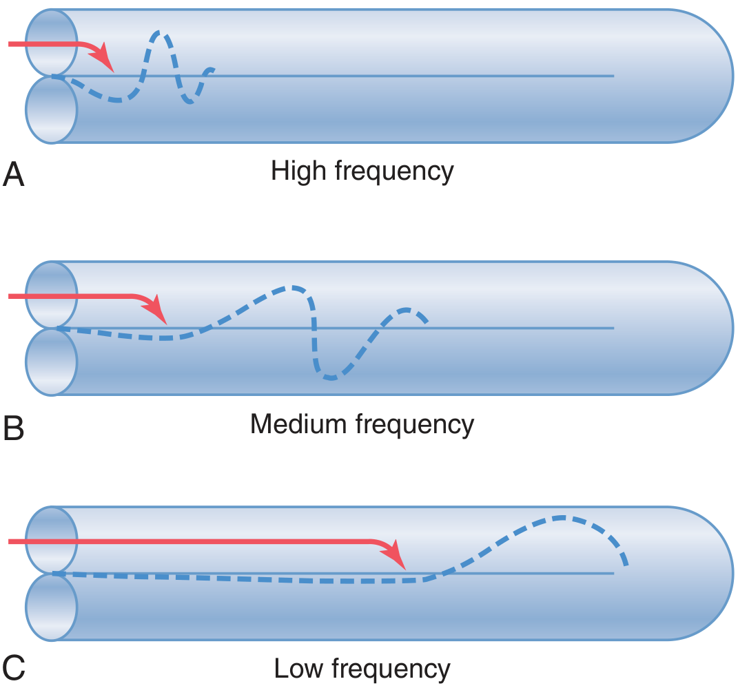
    elems.append(cap("Fig. 53.4 — Traveling waves along the basilar membrane. (A) High-frequency sound: wave dies near the base. "
                      "(B) Medium frequency: wave dies halfway. (C) Low frequency: wave travels the full length. (Guyton & Hall)"))
    elems.append(sp(1))

    elems.append(p("When the stapes pushes inward on the oval window:"))
    elems += bul([
        "Round window bulges outward (cochlea bounded by bone — fluid incompressible)",
        "A pressure wave initiates at the base of the basilar membrane and <b>travels</b> toward the helicotrema",
        "As the wave reaches the region of the membrane whose <b>natural resonant frequency matches the sound frequency</b>, it gains amplitude",
        "The membrane vibrates maximally at that point — energy is dissipated and the wave <b>dies</b>",
        "High-frequency waves die near the base; low-frequency waves travel the full length"
    ])
    elems.append(sp(0.5))
    elems.append(p("The wave travels <i>fast</i> near the base (high stiffness) and <i>slows</i> apically (decreasing stiffness). "
                   "This spreading prevents all high-frequency waves from bunching in the first millimeter."))
    elems.append(sp(1))
    elems.append(PageBreak())

    # ── 4. ORGAN OF CORTI ────────────────────────────────────────────────────
    elems.append(section_divider("4. ORGAN OF CORTI & SOUND TRANSDUCTION"))
    elems.append(sp(1))

    elems.append(h2("Structure of the Organ of Corti"))
    elems.append(p("The organ of Corti sits on the basilar membrane within the scala media and contains the receptor hair cells:"))
    elems.append(sp(0.5))

    hair_table = styled_table(
        ["Feature", "Inner Hair Cells", "Outer Hair Cells"],
        [
            ["Arrangement",         "Single row",            "3–4 rows"],
            ["Number",              "~3,500",                "~12,000"],
            ["Diameter",            "~12 μm",                "~8 μm"],
            ["Nerve fiber share",   "~90–95% of cochlear nerve endings", "~5–10%"],
            ["Primary function",    "Sound detection (main auditory signal)", "Amplification / 'tuning' of inner hair cells"],
        ],
        col_widths=[50*mm, 60*mm, 60*mm]
    )
    elems.append(hair_table)
    elems.append(sp(0.5))
    elems += bul([
        "<b>Tectorial membrane:</b> Gelatinous membrane overlying the hair cells; stereocilia are embedded in or touch it",
        "<b>Reticular lamina:</b> Rigid plate holding hair cells, supported by triangular rods of Corti on basilar fibers",
        "<b>Spiral ganglion (ganglion of Corti):</b> Located in the modiolus (central bony pillar); ~30,000 axons form the cochlear nerve"
    ])
    elems.append(sp(1))

    elems.append(h2("Mechanism of Hair Cell Excitation"))
    elems += bul([
        "Basilar membrane vibrates → reticular lamina rocks up/inward, then down/outward",
        "Stereocilia (stiff hairs on apical surface of hair cells) shear against tectorial membrane",
        "Bending toward <i>taller</i> stereocilia → tips of shorter cilia tugged outward → mechanical gating of K⁺ channels",
        "K⁺ rushes IN from high-K⁺ endolymph → cell <b>depolarizes</b>",
        "Depolarization opens voltage-gated <b>Ca²⁺ channels</b> → Ca²⁺ influx augments depolarization",
        "Ca²⁺ triggers release of <b>glutamate</b> (fast excitatory transmitter) at basal synapses",
        "Glutamate depolarizes cochlear nerve terminals → <b>action potentials</b> to CNS",
        "Bending in the opposite direction → <b>hyperpolarization</b>"
    ])
    elems.append(sp(1))

    elems.append(h2("The Endocochlear Potential"))
    elems.append(p("An electrical potential of <b>+80 mV</b> exists between endolymph (scala media) and perilymph, "
                   "generated by continual secretion of K⁺ by the <b>stria vascularis</b> (vascular strip on outer wall):"))
    elems += bul([
        "Endolymph: <b>high K⁺ (~150 mM), low Na⁺</b> — opposite of normal extracellular fluid",
        "Hair cell intracellular potential: –70 mV relative to perilymph, but <b>–150 mV</b> relative to endolymph",
        "This 150 mV gradient dramatically amplifies sensitivity — K⁺ rushes in powerfully upon channel opening",
        "The endocochlear potential is essential: drugs or disease damaging the stria vascularis cause profound hearing loss"
    ])
    elems.append(sp(1))
    elems.append(kf("Neurotransmitter: Glutamate. Depolarization = K⁺ in from endolymph. Endocochlear potential = +80 mV, generated by stria vascularis."))
    elems.append(sp(1))
    elems.append(PageBreak())

    # ── 5. CENTRAL AUDITORY PATHWAY ──────────────────────────────────────────
    elems.append(section_divider("5. CENTRAL AUDITORY PATHWAYS"))
    elems.append(sp(1))

    elems.append(h2("Ascending Pathway"))
    elems.append(p("Auditory signals ascend from the cochlea through bilateral relay stations to the temporal cortex:"))
    elems.append(sp(0.5))

    pathway_data = styled_table(
        ["Station", "Location", "Key Function"],
        [
            ["Spiral ganglion (CN VIII)", "Modiolus of cochlea", "First-order neurons; ~30,000 fibers in cochlear nerve"],
            ["Cochlear nuclei (dorsal & ventral)", "Upper medulla (pontomedullary junction)", "First brainstem relay; all cochlear fibers synapse here"],
            ["Superior olivary nucleus", "Lower pons", "First site of binaural convergence; sound localization"],
            ["Inferior colliculus", "Midbrain tectum", "Major auditory integration center; reflexive responses to sound"],
            ["Medial geniculate nucleus (MGN)", "Thalamus", "Relay to cortex; tonotopic organization maintained"],
            ["Primary auditory cortex (A1)", "Heschl's gyri, superior temporal plane", "Conscious hearing; frequency and intensity analysis"],
            ["Auditory association cortex", "Surrounding belt, Wernicke's area", "Interpretation of meaning of sounds / language"],
        ],
        col_widths=[50*mm, 55*mm, 65*mm]
    )
    elems.append(pathway_data)
    elems.append(sp(1))

    elems.append(h2("Sound Localization — Superior Olivary Nucleus"))
    elems.append(p("Two mechanisms detect sound direction, both processed initially in the superior olivary nucleus:"))
    elems.append(sp(0.5))

    loc_table = styled_table(
        ["Mechanism", "Neural Structure", "Best Frequency Range", "Principle"],
        [
            ["Interaural Time Difference (ITD)", "Medial superior olivary nucleus", "< 3,000 Hz",
             "Neurons with bilateral dendrites respond maximally to specific time lags between the two ears"],
            ["Interaural Level Difference (ILD)", "Lateral superior olivary nucleus", "> 3,000 Hz",
             "Head creates acoustic shadow at high frequencies; intensity difference between ears is compared"],
        ],
        col_widths=[42*mm, 45*mm, 28*mm, 55*mm]
    )
    elems.append(loc_table)
    elems.append(sp(0.5))
    elems += bul([
        "Direct frontal sound → simultaneous arrival at both ears → no time lag signal",
        "Pinna shape enables discrimination of elevation (up/down) and front/back by modifying frequency spectrum",
        "Bilateral destruction of auditory cortex → near-total loss of sound localization ability"
    ])
    elems.append(sp(1))

    elems.append(h2("Auditory Cortex"))
    elems += bul([
        "<b>Primary auditory cortex (areas 41, 42):</b> Heschl's gyri, superior temporal plane; tonotopic organization "
        "(high freq. posteriorly, low freq. anteriorly); detects frequency, intensity, and temporal patterns",
        "<b>Auditory association cortex:</b> Surrounding belt areas; integrates auditory patterns; required for meaning",
        "<b>Wernicke's area:</b> Posterior superior temporal gyrus; lesion → person hears words clearly but cannot interpret "
        "their meaning (<i>Wernicke's aphasia / receptive aphasia</i>)"
    ])
    elems.append(sp(1))
    elems.append(info_box("Clinical Note: Wernicke's Aphasia",
        ["Damage to Wernicke's area (posterior superior temporal gyrus) causes receptive aphasia.",
         "Patient can hear and repeat words perfectly but cannot understand their meaning.",
         "Differs from conductive or sensorineural deafness — the primary auditory cortex is intact."],
        bg=HexColor("#fff3e0"), title_color=GOLD))
    elems.append(PageBreak())

    return elems


# ─── PART II: VISION ──────────────────────────────────────────────────────────

def part2_vision(page_w):
    elems = []

    # Part banner
    data = [[Paragraph("PART II: PHYSIOLOGY OF VISION", ParagraphStyle(
        "pv", fontSize=20, textColor=WHITE, fontName="Helvetica-Bold",
        alignment=TA_CENTER, leading=26
    ))]]
    t = Table(data, colWidths=[170*mm])
    t.setStyle(TableStyle([
        ("BACKGROUND", (0,0), (-1,-1), TEAL),
        ("TOPPADDING",    (0,0), (-1,-1), 14),
        ("BOTTOMPADDING", (0,0), (-1,-1), 14),
    ]))
    elems.append(sp(1))
    elems.append(t)
    elems.append(sp(2))

    # Eye diagram
    img_eye = make_image("eye_retina", IMAGES["eye_retina"], page_w * 0.88, 130*mm)
    elems.append(img_eye)
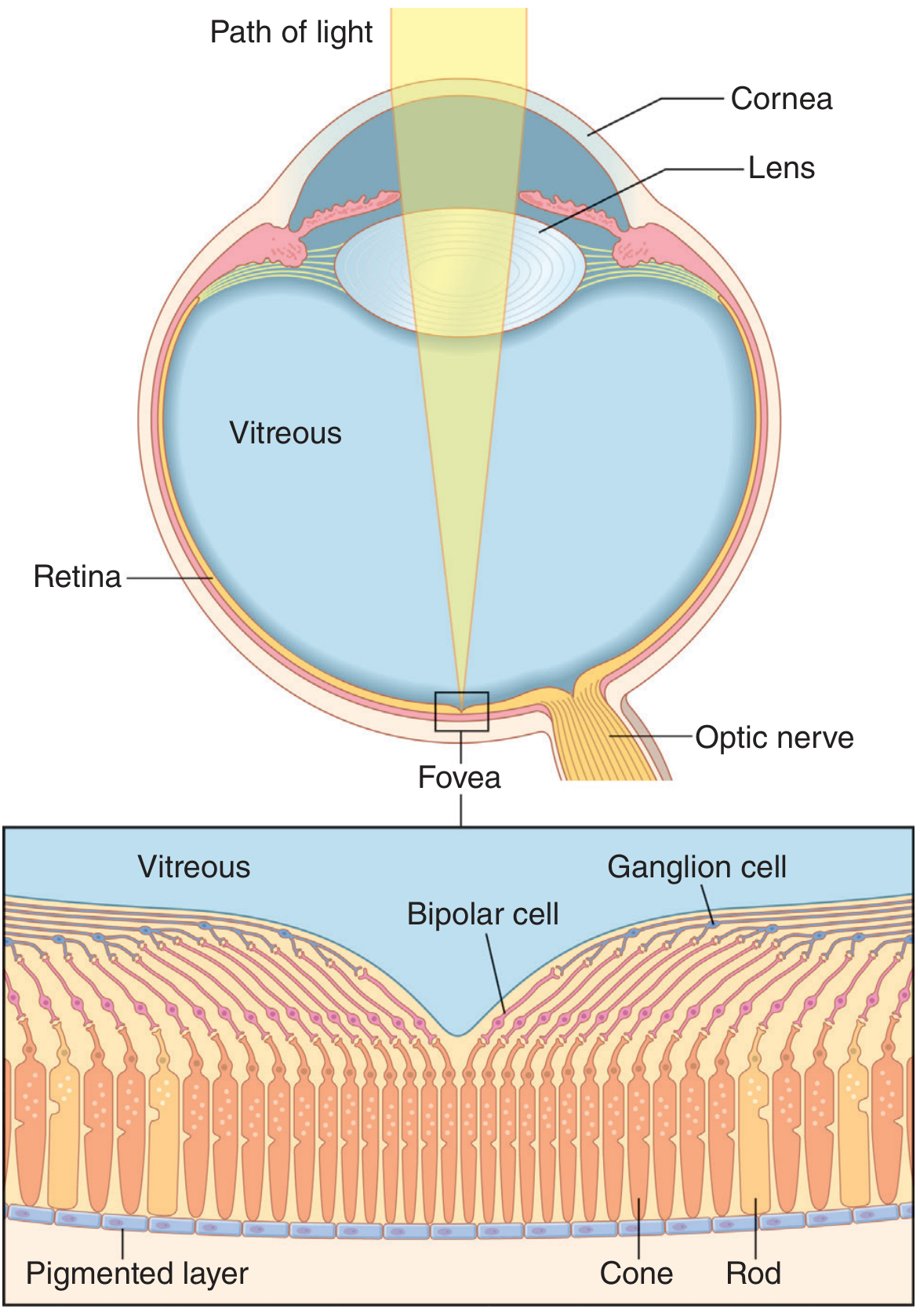
    elems.append(cap("Fig. 51.2 — Cross-section of the human eye showing path of light to the fovea. Inset: retinal layers at the fovea, "
                      "showing cones, bipolar cells, and ganglion cells displaced laterally. (Guyton & Hall)"))
    elems.append(sp(1))

    # ── 6. OPTICS ────────────────────────────────────────────────────────────
    elems.append(section_divider("6. OPTICS OF THE EYE", TEAL))
    elems.append(sp(1))

    elems.append(h2("Refracting Surfaces"))
    elems.append(p("Light is focused onto the retina by four refracting surfaces. The <b>cornea</b> provides the majority of the eye's refractive power:"))
    elems.append(sp(0.5))

    refract_table = styled_table(
        ["Refracting Surface", "Power (Diopters)", "Notes"],
        [
            ["Anterior corneal surface", "~+43 D", "Most powerful surface; air-cornea interface (greatest RI difference)"],
            ["Anterior lens surface",    "~+15 D", "Increases during accommodation"],
            ["Posterior lens surface",   "~+5 D",  "Increases during accommodation"],
            ["Total (relaxed eye)",      "~+59 D", "Focal point falls on retina (~17 mm behind cornea)"],
            ["Total (max accommodation)","~+70 D", "Maximum near-focus power"],
        ],
        col_widths=[55*mm, 30*mm, 85*mm]
    )
    elems.append(refract_table)
    elems.append(sp(1))

    elems.append(h2("Accommodation"))
    elems.append(p("To focus on <b>near objects</b>, the eye increases its refractive power by rounding the lens:"))
    elems += bul([
        "Near object → ciliary muscle <b>contracts</b> → zonular fibers <b>relax</b> → lens rounds up (increases curvature)",
        "Far object → ciliary muscle <b>relaxes</b> → zonular fibers <b>tighten</b> → lens flattens",
        "<b>Near point:</b> Closest distance at which the eye can focus clearly; ~8–9 cm in young adults",
        "<b>Presbyopia:</b> Age-related loss of accommodation (lens hardens, loses elasticity); near point recedes progressively",
        "Neural pathway: Brodmann areas 18 and 19 → pretectal area → Edinger-Westphal nucleus → ciliary ganglion → ciliary muscle"
    ])
    elems.append(sp(1))

    # ── 7. REFRACTIVE ERRORS ─────────────────────────────────────────────────
    elems.append(section_divider("7. REFRACTIVE ERRORS", TEAL))
    elems.append(sp(1))

    rf_table = styled_table(
        ["Condition", "Defect", "Correction", "Key Point"],
        [
            ["Emmetropia", "Normal — parallel rays focus on retina", "None", "Ideal refraction"],
            ["Myopia (nearsightedness)", "Eyeball too long OR cornea too curved; parallel rays focus in FRONT of retina",
             "Concave (diverging) lens", "Can see near objects clearly; far objects blurry"],
            ["Hyperopia (farsightedness)", "Eyeball too short; parallel rays focus BEHIND retina",
             "Convex (converging) lens", "Young patients may accommodate to overcome mild hyperopia"],
            ["Astigmatism", "Corneal curvature unequal in two planes; different focal lengths at 90°",
             "Cylindrical lens (axis-specific)", "Cannot be compensated by accommodation (both planes require different power)"],
            ["Presbyopia", "Lens loses elasticity with age; accommodative amplitude decreases",
             "Convex reading glasses (bifocals)", "Near point recedes with age; universal with aging"],
        ],
        col_widths=[32*mm, 48*mm, 38*mm, 52*mm]
    )
    elems.append(rf_table)
    elems.append(sp(1))
    elems.append(PageBreak())

    # ── 8. RETINA ─────────────────────────────────────────────────────────────
    elems.append(section_divider("8. RETINA — FUNCTIONAL ANATOMY", TEAL))
    elems.append(sp(1))

    elems.append(h2("Layers of the Retina (outer → inner, from pigment layer to vitreous)"))
    elems.append(sp(0.5))

    layer_table = styled_table(
        ["Layer", "Cells / Components", "Function"],
        [
            ["1. Pigmented epithelium", "Melanin-containing cells", "Absorbs scattered light; stores vitamin A (retinal); phagocytoses shed outer segments"],
            ["2. Photoreceptor layer", "Rod and cone outer segments", "Phototransduction — light → electrical signal"],
            ["3. Outer nuclear layer", "Nuclei of rods and cones", "Cellular bodies of photoreceptors"],
            ["4. Outer plexiform layer", "Synapses", "Connections between photoreceptors and bipolar/horizontal cells"],
            ["5. Inner nuclear layer", "Bipolar, horizontal, amacrine cells", "Initial signal processing; lateral inhibition"],
            ["6. Inner plexiform layer", "Synapses", "Connections between bipolar/amacrine and ganglion cells"],
            ["7. Ganglion cell layer", "Retinal ganglion cells (RGCs)", "Output neurons of retina; axons form the optic nerve"],
            ["8. Nerve fiber layer", "Axons of RGCs", "Converge at optic disc to form optic nerve"],
        ],
        col_widths=[42*mm, 48*mm, 80*mm]
    )
    elems.append(layer_table)
    elems.append(sp(0.5))
    elems.append(info_box("Fovea — Center of Acute Vision",
        ["Location: Center of retina, ~0.3 mm diameter",
         "Composition: Almost entirely cones (no rods)",
         "Special feature: All overlying neural layers displaced laterally — light reaches cones directly",
         "Cones: Very slender (1.5 μm) and densely packed → highest acuity",
         "No blood vessels in central fovea — avascular zone"],
        bg=ACCENT))
    elems.append(sp(1))

    # ── 9. PHOTORECEPTORS ─────────────────────────────────────────────────────
    elems.append(section_divider("9. PHOTORECEPTORS: RODS & CONES", TEAL))
    elems.append(sp(1))

    # Rod/Cone diagram
    img_rc = make_image("rod_cone", IMAGES["rod_cone"], page_w * 0.45, 120*mm)
    # Put image alongside table
    rc_table = styled_table(
        ["Feature", "Rods", "Cones"],
        [
            ["Number in retina", "~100 million", "~6 million"],
            ["Location", "Periphery; absent from fovea", "Concentrated in fovea; scattered peripherally"],
            ["Photochemical", "Rhodopsin", "3 types of color pigments"],
            ["Sensitivity to light", "Very high (single photon)", "Lower (require brighter light)"],
            ["Color discrimination", "None", "Full color vision (3-color trichromacy)"],
            ["Visual acuity", "Low", "High (especially foveal cones)"],
            ["Vision type", "Scotopic (dim light / night)", "Photopic (daylight / color)"],
            ["Outer segment shape", "Long cylinder", "Tapered cone"],
        ],
        col_widths=[42*mm, 63*mm, 63*mm]
    )
    elems.append(Table(
        [[img_rc, rc_table]],
        colWidths=[page_w*0.42, page_w*0.58],
        style=TableStyle([
            ("VALIGN", (0,0), (-1,-1), "TOP"),
            ("LEFTPADDING", (0,0), (-1,-1), 2),
            ("RIGHTPADDING", (0,0), (-1,-1), 2),
            ("TOPPADDING", (0,0), (-1,-1), 0),
        ])
    ))
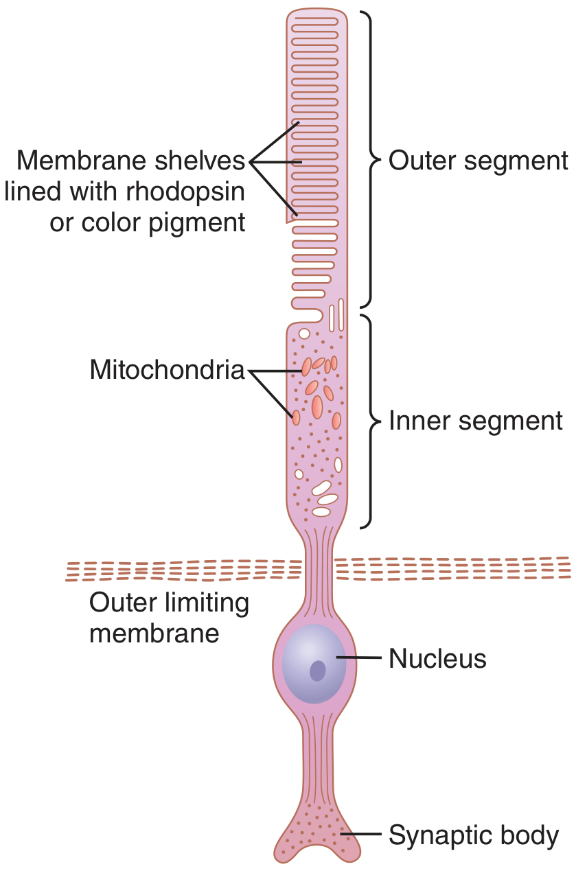
    elems.append(cap("Fig. 51.3 — Schematic of rod/cone structure. Outer segment membrane shelves lined with rhodopsin or color pigment. (Guyton & Hall)"))
    elems.append(sp(1))

    elems.append(h3("Four Functional Segments of Each Photoreceptor"))
    elems += bul([
        "<b>Outer segment:</b> Stacks of membrane disks containing photopigment (rhodopsin in rods; color pigment in cones) — site of phototransduction",
        "<b>Inner segment:</b> Contains mitochondria for metabolic energy production",
        "<b>Nucleus:</b> In the outer nuclear layer",
        "<b>Synaptic body:</b> Synapses with bipolar cells (and horizontal cells)"
    ])
    elems.append(sp(1))

    # ── 10. PHOTOTRANSDUCTION ─────────────────────────────────────────────────
    elems.append(section_divider("10. PHOTOTRANSDUCTION", TEAL))
    elems.append(sp(1))

    elems.append(h2("The Rhodopsin Cycle (Rods)"))
    elems += bul([
        "<b>Rhodopsin = opsin</b> (G-protein–coupled receptor protein) + <b>retinal</b> (vitamin A aldehyde derivative, 11-cis form)",
        "Light → retinal isomerizes from <b>11-cis → all-trans</b> configuration",
        "Activated rhodopsin (metarhodopsin II) → activates <b>transducin</b> (Gα subunit)",
        "Transducin activates <b>phosphodiesterase (PDE)</b>",
        "PDE hydrolyzes <b>cGMP → 5'-GMP</b> (reduces cGMP levels)",
        "Reduced cGMP → <b>cGMP-gated Na⁺/Ca²⁺ channels close</b>",
        "Less Na⁺ influx → membrane <b>hyperpolarizes</b> (–40 mV → –70 mV)",
        "Hyperpolarization → reduced release of <b>glutamate</b> from synaptic body → ON-bipolar cells depolarize"
    ])
    elems.append(sp(0.5))
    elems.append(info_box("Dark Current vs. Light Response",
        ["In the DARK: cGMP levels are high → cGMP-gated channels OPEN → Na⁺/Ca²⁺ flow in continuously ('dark current') → cell is DEPOLARIZED (~−40 mV) → steady glutamate release",
         "In the LIGHT: cGMP falls → channels CLOSE → cell HYPERPOLARIZES (~−70 mV) → glutamate release DECREASES",
         "KEY: Photoreceptors are DEPOLARIZED at rest and HYPERPOLARIZE in response to light — opposite of most neurons!"],
        bg=HexColor("#fff3e0"), title_color=RED_DARK))
    elems.append(sp(1))

    elems.append(h2("Light and Dark Adaptation"))
    elems += bul([
        "<b>Dark adaptation:</b> As rhodopsin regenerates in the dark, sensitivity increases over ~20–30 min (rods reach full sensitivity later than cones)",
        "<b>Light adaptation:</b> Bright light bleaches most rhodopsin → rapid decrease in sensitivity; pupils constrict; cone pigments decrease",
        "Rods are ~500–1000× more sensitive than cones; rods are saturated in bright light"
    ])
    elems.append(sp(1))

    # ── 11. COLOR VISION ──────────────────────────────────────────────────────
    elems.append(section_divider("11. COLOR VISION", TEAL))
    elems.append(sp(1))

    elems.append(p("Three types of cones, each containing a different photopigment with a different spectral sensitivity peak:"))
    elems.append(sp(0.5))

    color_table = styled_table(
        ["Cone Type", "Peak Sensitivity", "Commonly Called", "Detects"],
        [
            ["S-cones (short wavelength)", "~445 nm", "Blue cones", "Blue / violet light"],
            ["M-cones (medium wavelength)", "~535 nm", "Green cones", "Green / yellow-green light"],
            ["L-cones (long wavelength)", "~570 nm", "Red cones", "Red / orange light"],
        ],
        col_widths=[50*mm, 35*mm, 35*mm, 50*mm]
    )
    elems.append(color_table)
    elems.append(sp(0.5))
    elems += bul([
        "All colors are perceived as <b>ratios of stimulation</b> of the three cone types (<i>trichromacy / Young-Helmholtz theory</i>)",
        "Color opponent channels in the retina: red-green and blue-yellow (opponent process theory)",
        "<b>Red-green color blindness</b> (deuteranopia/protanopia): Most common; X-linked; absence of M or L cones",
        "<b>Tritanopia (blue-yellow blindness):</b> Rare; autosomal; S-cone absence"
    ])
    elems.append(sp(1))
    elems.append(PageBreak())

    # ── 12. RETINAL NEURAL PROCESSING ────────────────────────────────────────
    elems.append(section_divider("12. RETINAL NEURAL PROCESSING", TEAL))
    elems.append(sp(1))

    elems.append(h2("Lateral Inhibition and Center-Surround Receptive Fields"))
    elems.append(p("Retinal ganglion cells have circular receptive fields with opposing center and surround:"))
    elems.append(sp(0.5))

    cs_table = styled_table(
        ["Cell Type", "Center response", "Surround response", "Function"],
        [
            ["ON-center ganglion cell",  "Excited by light",   "Inhibited by light",  "Signals bright spots on dark background"],
            ["OFF-center ganglion cell", "Inhibited by light", "Excited by light",    "Signals dark spots on bright background"],
        ],
        col_widths=[45*mm, 35*mm, 35*mm, 55*mm]
    )
    elems.append(cs_table)
    elems.append(sp(0.5))
    elems += bul([
        "<b>Horizontal cells:</b> Mediate lateral inhibition in the outer plexiform layer (between photoreceptors and bipolar cells)",
        "<b>Amacrine cells:</b> Mediate lateral interactions in the inner plexiform layer; some detect directional motion",
        "Center-surround antagonism enhances <b>edge detection and contrast</b>"
    ])
    elems.append(sp(1))

    elems.append(h2("Two Types of Retinal Ganglion Cells"))
    elems.append(sp(0.5))

    rg_table = styled_table(
        ["Cell Type", "Size", "Conduction Speed", "Signal Content", "Project to LGN Layer"],
        [
            ["M-type (magnocellular)", "Large soma", "Fast", "Motion, coarse form, depth; black & white; no color", "Layers 1 & 2 (magnocellular)"],
            ["P-type (parvocellular)", "Small soma", "Slow", "Fine detail, color, texture; sustained response",  "Layers 3–6 (parvocellular)"],
        ],
        col_widths=[30*mm, 18*mm, 22*mm, 55*mm, 45*mm]
    )
    elems.append(rg_table)
    elems.append(sp(1))
    elems.append(PageBreak())

    # ── 13. CENTRAL VISUAL PATHWAYS ──────────────────────────────────────────
    elems.append(section_divider("13. CENTRAL VISUAL PATHWAYS: RETINA TO CORTEX", TEAL))
    elems.append(sp(1))

    # Visual pathway diagram
    img_vp = make_image("visual_pathway", IMAGES["visual_pathway"], page_w * 0.90, 120*mm)
    elems.append(img_vp)
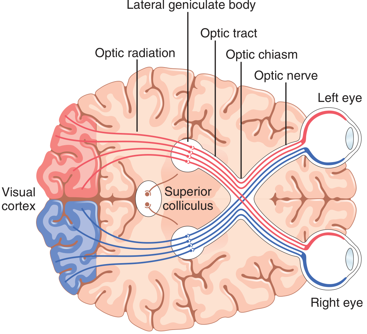
    elems.append(cap("Fig. 52.1 — Principal visual pathways: optic nerve → optic chiasm → optic tract → lateral geniculate body → "
                      "optic radiation → visual cortex (occipital lobe). Note decussation of nasal fibers at the chiasm. (Guyton & Hall)"))
    elems.append(sp(1))

    elems.append(h2("The Complete Pathway"))
    pathway_vis = styled_table(
        ["Structure", "Location", "Key Feature"],
        [
            ["Optic nerve (CN II)", "From retina to optic chiasm", "Contains ~1.2 million axons from retinal ganglion cells; no synapse"],
            ["Optic chiasm", "At base of brain, above pituitary", "Nasal retinal fibers CROSS; temporal fibers remain ipsilateral"],
            ["Optic tract", "Chiasm to LGN", "Contains fibers from BOTH eyes representing one visual hemifield"],
            ["Lateral geniculate nucleus (LGN)", "Dorsal thalamus", "6-layer relay; keeps M and P pathways; keeps two eyes separate"],
            ["Optic radiation (geniculocalcarine tract)", "From LGN to occipital lobe", "Meyer's loop (inferior) carries upper visual field; superior fibers carry lower field"],
            ["Primary visual cortex (V1 / area 17)", "Calcarine fissure, medial occipital lobe", "Retinotopic map; fovea magnified; edge and orientation detection"],
        ],
        col_widths=[45*mm, 45*mm, 80*mm]
    )
    elems.append(pathway_vis)
    elems.append(sp(1))

    elems.append(h2("The Optic Chiasm — Decussation Rules"))
    elems.append(p("The partial decussation at the optic chiasm creates binocular representation of each visual hemifield in the contralateral hemisphere:"))
    elems.append(sp(0.5))

    chiasm_table = styled_table(
        ["Retinal Fiber Origin", "Crosses at Chiasm?", "Joins Which Optic Tract?", "Represents"],
        [
            ["Nasal (medial) retina — right eye", "YES — crosses to LEFT", "Left optic tract", "Right visual field of right eye"],
            ["Temporal (lateral) retina — right eye", "NO — stays right", "Right optic tract", "Left visual field of right eye"],
            ["Nasal (medial) retina — left eye", "YES — crosses to RIGHT", "Right optic tract", "Left visual field of left eye"],
            ["Temporal (lateral) retina — left eye", "NO — stays left", "Left optic tract", "Right visual field of left eye"],
        ],
        col_widths=[50*mm, 32*mm, 40*mm, 48*mm]
    )
    elems.append(chiasm_table)
    elems.append(sp(0.5))
    elems.append(info_box("Result of Decussation",
        ["RIGHT optic tract = information from the LEFT visual field from BOTH eyes",
         "LEFT optic tract = information from the RIGHT visual field from BOTH eyes",
         "Lesion of ONE optic tract → contralateral homonymous hemianopia"],
        bg=ACCENT))
    elems.append(sp(1))
    elems.append(PageBreak())

    # ── 14. LGN ──────────────────────────────────────────────────────────────
    elems.append(section_divider("14. LATERAL GENICULATE NUCLEUS (LGN)", TEAL))
    elems.append(sp(1))

    elems.append(p("The LGN (also called lateral geniculate body) is the main thalamic relay for vision. It has <b>6 layers</b>:"))
    elems.append(sp(0.5))

    lgn_table = styled_table(
        ["Layer", "Cell Type", "Eye Input", "Pathway"],
        [
            ["1",   "Magnocellular (large)", "Contralateral eye", "M pathway (motion, coarse form)"],
            ["2",   "Magnocellular (large)", "Ipsilateral eye",   "M pathway"],
            ["3",   "Parvocellular (small)", "Ipsilateral eye",   "P pathway (color, fine detail)"],
            ["4",   "Parvocellular (small)", "Contralateral eye", "P pathway"],
            ["5",   "Parvocellular (small)", "Ipsilateral eye",   "P pathway"],
            ["6",   "Parvocellular (small)", "Contralateral eye", "P pathway"],
        ],
        col_widths=[15*mm, 40*mm, 40*mm, 75*mm]
    )
    elems.append(lgn_table)
    elems.append(sp(0.5))

    elems.append(h3("Functions of the LGN"))
    elems += bul([
        "<b>Relay:</b> Point-to-point transmission from retina to V1 with high spatial fidelity (retinotopic map preserved)",
        "<b>Separation:</b> Keeps the two eyes' signals in separate layers; keeps M and P pathways separate",
        "<b>Gating:</b> Reticular formation inputs can amplify or suppress visual signals (attention/arousal modulation)",
        "Both hemispheres receive input from BOTH eyes — bilateral representation after the chiasm"
    ])
    elems.append(sp(1))

    # ── 15. PRIMARY VISUAL CORTEX ─────────────────────────────────────────────
    elems.append(section_divider("15. PRIMARY VISUAL CORTEX (V1)", TEAL))
    elems.append(sp(1))

    elems.append(h2("Location and Organization"))
    elems += bul([
        "Located in the <b>calcarine fissure</b>, medial surface of the <b>occipital lobe</b>",
        "Also called: <b>striate cortex, area 17, Brodmann area 17</b>",
        "<b>Retinotopic organization:</b> Every point in the visual field maps to a specific point in V1",
        "<b>Cortical magnification:</b> The fovea (small area of retina) occupies a disproportionately large area of V1",
        "Upper visual field → lower lip of calcarine fissure; lower visual field → upper lip"
    ])
    elems.append(sp(1))

    elems.append(h2("Feature Detection in V1"))
    feature_table = styled_table(
        ["Feature Detected", "Cell Type", "Mechanism"],
        [
            ["Contrast / edges", "All V1 neurons", "Respond to transitions in luminance (borders); not to uniform illumination"],
            ["Orientation (line direction)", "Simple cells", "Linear arrays of mutually inhibiting ON/OFF center cells; each cell responds to ONE orientation"],
            ["Moving oriented edges", "Complex cells", "Respond to oriented edges anywhere in receptive field; direction-selective subgroup"],
            ["Ocular dominance", "Ocular dominance columns", "Alternating cortical columns respond preferentially to left or right eye"],
            ["Spatial frequency", "Gratings of specific widths", "Tuned for coarse vs. fine patterns in the image"],
        ],
        col_widths=[45*mm, 35*mm, 90*mm]
    )
    elems.append(feature_table)
    elems.append(sp(1))

    # ── 16. DORSAL & VENTRAL STREAMS ──────────────────────────────────────────
    elems.append(section_divider("16. DORSAL & VENTRAL VISUAL STREAMS", TEAL))
    elems.append(sp(1))

    elems.append(p("From V1, visual signals diverge into two parallel processing streams for different aspects of vision:"))
    elems.append(sp(0.5))

    stream_table = styled_table(
        ["Stream", "Nickname", "Pathway", "Analyzes", "Driven by"],
        [
            ["Dorsal stream", '"Where / How"', "V1 → Posterior parietal cortex (occipitoparietal)",
             "3-D position, spatial location, gross form, motion, visually guided action",
             "M-type ganglion cells (fast, no color)"],
            ["Ventral stream", '"What"', "V1 → Inferior temporal cortex (occipitotemporal)",
             "Object identity, fine detail, color, texture, face recognition, reading",
             "P-type ganglion cells (slow, color)"],
        ],
        col_widths=[25*mm, 22*mm, 45*mm, 48*mm, 30*mm]
    )
    elems.append(stream_table)
    elems.append(sp(0.5))
    elems.append(info_box("Clinical Relevance of the Two Streams",
        ["Dorsal stream lesion (parietal): Optic ataxia — patient can identify objects but cannot reach for them accurately.",
         "Ventral stream lesion (temporal): Visual agnosia — patient can navigate the environment but cannot recognize or name objects.",
         "Prosopagnosia: Selective lesion of face-recognition area in inferior temporal cortex (fusiform face area)."],
        bg=HexColor("#fff3e0"), title_color=RED_DARK))
    elems.append(sp(1))

    # ── 17. PUPILLARY REFLEXES ────────────────────────────────────────────────
    elems.append(section_divider("17. PUPILLARY REFLEXES", TEAL))
    elems.append(sp(1))

    elems.append(h2("Pupillary Light Reflex"))
    elems += bul([
        "<b>Pathway:</b> Retina → Optic nerve → Pretectal nucleus (midbrain) → Edinger-Westphal nucleus → Ciliary ganglion → Constrictor pupillae → <b>Miosis</b>",
        "Both pupils constrict when light enters either eye (<b>consensual reflex</b>)",
        "Pupil range: <b>1.5 mm</b> (max miosis) to <b>8 mm</b> (max mydriasis)",
        "This provides up to <b>30-fold change</b> in light reaching the retina (squares of diameters)",
        "Sympathetic nerves → radial dilator muscle → <b>mydriasis</b>"
    ])
    elems.append(sp(1))

    elems.append(h2("Clinical Pupillary Syndromes"))
    pupil_table = styled_table(
        ["Syndrome / Sign", "Finding", "Lesion Site", "Cause"],
        [
            ["Argyll Robertson pupil", "No light reflex; intact accommodation reflex; small pupil",
             "Pretectal area (bilateral)", "Neurosyphilis, chronic alcoholism, MS, Lyme disease"],
            ["Horner syndrome", "Ptosis + miosis + anhidrosis + enophthalmos",
             "Interruption of cervical sympathetic chain", "Pancoast tumor, carotid dissection, brainstem stroke"],
            ["Fixed dilated pupil", "No response to light; mydriasis",
             "CN III compression (parasympathetic fibers on outside)", "Transtentorial herniation, posterior communicating artery aneurysm"],
            ["Relative afferent pupillary defect (RAPD)", "Consensual reflex intact; direct reflex diminished in affected eye",
             "Optic nerve or retina (afferent limb)", "Optic neuritis, severe retinal disease"],
        ],
        col_widths=[40*mm, 48*mm, 40*mm, 42*mm]
    )
    elems.append(pupil_table)
    elems.append(sp(1))
    elems.append(PageBreak())

    return elems


# ─── QUICK REFERENCE & CLINICAL TABLES ───────────────────────────────────────

def quick_reference():
    elems = []

    data = [[Paragraph("QUICK REFERENCE TABLES & CLINICAL CORRELATIONS", ParagraphStyle(
        "qr", fontSize=18, textColor=WHITE, fontName="Helvetica-Bold",
        alignment=TA_CENTER, leading=24
    ))]]
    t = Table(data, colWidths=[170*mm])
    t.setStyle(TableStyle([
        ("BACKGROUND", (0,0), (-1,-1), HexColor("#2d3748")),
        ("TOPPADDING",    (0,0), (-1,-1), 12),
        ("BOTTOMPADDING", (0,0), (-1,-1), 12),
    ]))
    elems.append(sp(1))
    elems.append(t)
    elems.append(sp(2))

    # ── Hearing summary ───────────────────────────────────────────────────────
    elems.append(h1("Hearing: High-Yield Summary"))
    h_summary = styled_table(
        ["Topic", "Key Fact (Guyton & Hall)"],
        [
            ["Impedance matching", "~22-fold force amplification; tympanic membrane (55 mm²) → stapes (3.2 mm²) × lever (1.3×)"],
            ["Efficiency range", "50–75% for 300–3000 Hz (speech range)"],
            ["Without ossicles", "15–20 dB hearing loss (direct air conduction)"],
            ["Attenuation reflex latency", "40–60 ms; protects against sustained noise, NOT impulse sounds"],
            ["Basilar membrane — base", "High frequency (~20,000 Hz); narrow, stiff fibers"],
            ["Basilar membrane — apex", "Low frequency (~20 Hz); wide, floppy fibers"],
            ["Inner hair cells", "~3,500; single row; receive 90–95% of cochlear nerve endings"],
            ["Outer hair cells", "~12,000; 3–4 rows; 'tuning' via retrograde efferents"],
            ["Endocochlear potential", "+80 mV (endolymph vs. perilymph); generated by stria vascularis"],
            ["Hair cell membrane potential", "–70 mV vs. perilymph; –150 mV vs. endolymph"],
            ["Neurotransmitter at synapse", "Glutamate"],
            ["Endolymph composition", "High K⁺, low Na⁺ (opposite of perilymph)"],
            ["Cochlear nerve fibers", "~30,000 axons from spiral ganglion"],
            ["Sound localization — time lag", "Medial superior olivary nucleus; best below 3,000 Hz"],
            ["Sound localization — intensity", "Lateral superior olivary nucleus; best above 3,000 Hz"],
            ["Wernicke's area", "Posterior superior temporal gyrus; receptive aphasia if damaged"],
            ["Primary auditory cortex", "Heschl's gyri (Brodmann areas 41, 42); tonotopic"],
        ],
        col_widths=[70*mm, 100*mm]
    )
    elems.append(h_summary)
    elems.append(sp(2))

    # ── Vision summary ────────────────────────────────────────────────────────
    elems.append(h1("Vision: High-Yield Summary"))
    v_summary = styled_table(
        ["Topic", "Key Fact (Guyton & Hall)"],
        [
            ["Cornea refractive power", "~+43 diopters (most of eye's focusing power)"],
            ["Total eye power (relaxed)", "~+59 diopters"],
            ["Total eye power (max accommodation)", "~+70 diopters"],
            ["Fovea diameter", "~0.3 mm; all cones; no rods; no overlying neurons"],
            ["Rods — number", "~100 million; periphery; scotopic (dim light) vision"],
            ["Cones — number", "~6 million; concentrated in fovea; photopic/color vision"],
            ["Photochemical in rods", "Rhodopsin (opsin + 11-cis retinal)"],
            ["Light causes in photoreceptors", "Hyperpolarization (not depolarization!)"],
            ["Dark current", "Na⁺/Ca²⁺ in via cGMP-gated channels in the dark; closed by light"],
            ["Cone peak sensitivities", "Blue (S): 445 nm; Green (M): 535 nm; Red (L): 570 nm"],
            ["Optic chiasm rule", "Nasal retinal fibers cross; temporal fibers stay ipsilateral"],
            ["Each optic tract represents", "Contralateral visual field from BOTH eyes"],
            ["LGN layers 1 & 2", "Magnocellular (M pathway): motion, coarse form"],
            ["LGN layers 3–6", "Parvocellular (P pathway): color, fine detail"],
            ["Primary visual cortex", "Calcarine fissure, occipital lobe (area 17/striate cortex)"],
            ["Dorsal stream ('Where/How')", "V1 → Posterior parietal cortex; spatial location, motion"],
            ["Ventral stream ('What')", "V1 → Inferior temporal cortex; object identity, color"],
            ["Pupillary light reflex arc", "Retina → Pretectum → Edinger-Westphal → ciliary ganglion → miosis"],
            ["Pupil range", "1.5 mm (miosis) to 8 mm (mydriasis) = 30-fold light change"],
        ],
        col_widths=[70*mm, 100*mm]
    )
    elems.append(v_summary)
    elems.append(sp(2))

    # ── Visual field defects ──────────────────────────────────────────────────
    elems.append(h1("Visual Field Defects — Lesion Localization"))
    vfd_table = styled_table(
        ["Lesion Site", "Visual Field Defect", "Clinical Clue"],
        [
            ["One optic nerve", "Monocular blindness (ipsilateral eye only)", "Total loss one eye; other eye normal"],
            ["Optic chiasm (central)", "Bitemporal hemianopia — both temporal fields lost",
             "Classic: pituitary adenoma compressing chiasm from below"],
            ["Optic chiasm (lateral)", "Monocular nasal hemianopia (rare)", "Carotid aneurysm compressing lateral chiasm"],
            ["Optic tract (one side)", "Contralateral homonymous hemianopia (incongruous)",
             "Left optic tract → right homonymous hemianopia"],
            ["Temporal lobe optic radiation (Meyer's loop)", "Contralateral superior quadrantanopia ('pie in the sky')",
             "Upper visual field fibers loop into temporal lobe"],
            ["Parietal lobe optic radiation", "Contralateral inferior quadrantanopia ('pie on the floor')",
             "Inferior visual field fibers in parietal lobe"],
            ["Occipital cortex (V1)", "Contralateral homonymous hemianopia WITH macular sparing",
             "Posterior cerebral artery stroke; macula has dual blood supply"],
            ["Occipital pole only", "Contralateral homonymous scotoma (central field loss)",
             "Affects the large foveal representation at the occipital pole"],
        ],
        col_widths=[48*mm, 62*mm, 60*mm]
    )
    elems.append(vfd_table)
    elems.append(sp(2))

    # ── Memory mnemonics ──────────────────────────────────────────────────────
    elems.append(h1("Memory Aids"))
    elems.append(info_box("Mnemonics for Exam",
        [
            "OSSICLES order lateral to medial: MIS — Malleus, Incus, Stapes",
            "BASILAR MEMBRANE frequency: BASE = HIGH freq (Stiff = Short wavelength); APEX = LOW freq (Floppy = Far waves travel)",
            "HAIR CELL depolarization: K+ rushes IN from K+-rich endolymph → opens like a gate when pushed toward taller cilia",
            "OPTIC CHIASM: Nasal fibres cross (N = No home), temporal fibres stay (T = Temporal = 'To the same side')",
            "LGN layers: 1,2 = Magno (M for Motion); 3,4,5,6 = Parvo (P for Precise colour)",
            "DORSAL = 'WHERE' (Parietal = spatial); VENTRAL = 'WHAT' (Temporal = object identity)",
            "ARGYLL ROBERTSON: 'Prostitute's pupil' — accommodates but does not react (to light) — syphilis",
            "HORNER's triad: Ptosis + Miosis + Anhidrosis (lost sympathetic to eye, lid, face)",
        ],
        bg=HexColor("#e8f5e9"), title_color=GREEN_DK))
    elems.append(sp(2))

    return elems


# ═══════════════════════════════════════════════════════════════════════════════
#  ASSEMBLE AND BUILD
# ═══════════════════════════════════════════════════════════════════════════════

def build():
    print("Downloading images...")
    for k, url in IMAGES.items():
        download_image(k, url)

    print("Building PDF...")
    doc = MyDocTemplate(
        OUTPUT,
        pagesize=A4,
        topMargin=22*mm, bottomMargin=16*mm,
        leftMargin=20*mm, rightMargin=20*mm,
        title="Physiology of Hearing & Vision — Study Guide",
        author="Guyton and Hall Textbook of Medical Physiology",
    )

    page_w = A4[0] - 40*mm   # usable width

    story = []
    story += cover_page()
    story += toc_section()
    story += part1_hearing(page_w)
    story += part2_vision(page_w)
    story += quick_reference()

    doc.build(story, onFirstPage=on_page, onLaterPages=on_page)
    print(f"\n✓ PDF saved to: {OUTPUT}")

if __name__ == "__main__":
    build()