CT ABDOMEN CONTRAST AND ABDOMEN TRIPLE PHASE

Reading File

CT abdomen with contrast and triple-phase CT are standard radiology techniques for abdominal imaging. Here is a quick overview while I search the textbooks for detailed content.

CT Abdomen Contrast: Uses intravenous iodinated contrast to enhance vascular structures and organs, improving detection of lesions, inflammation, and vascular pathology.

Triple Phase CT: Refers to three imaging phases - arterial (~25-35 sec), portal venous (~60-70 sec), and delayed (~3-5 min) - particularly used for liver lesion characterization and vascular evaluation.

Searching sources...

Finding Sources

Searching the Web

CT abdomen contrast vs triple phase CT indications technique phases explained

Finding Sources

Reading Web Page

https://litfl.com/abdominal-ct-phases

Reading File

Finding Sources

Reading File

Loading Image

Reading File

Here is a thorough, well-structured guide to CT Abdomen with Contrast and Triple-Phase CT of the Abdomen, synthesized from authoritative radiology and surgical textbooks.

CT Abdomen with Contrast

What Is It?

CT abdomen with contrast uses intravenous (IV) iodinated contrast medium to enhance vascular structures, organs, and pathological lesions. Oral contrast may be added to opacify the bowel lumen. The study dramatically improves detection and characterization of lesions compared to non-contrast CT alone.

Indications

Abdominal pain (suspected appendicitis, diverticulitis, bowel obstruction, perforation)
Trauma evaluation (hepatic, splenic, renal, mesenteric injuries)
Detection and staging of abdominal tumors, enlarged lymph nodes, metastases
Fluid collections (abscess, hemorrhage, ascites)
Vascular pathology (mesenteric ischemia, aortic aneurysm, venous thrombosis)
Air outside the GI tract (pneumoperitoneum)

Standard Technique

Parameter	Detail
Patient position	Supine, arms elevated
Scan extent	Diaphragm to symphysis pubis
Slice thickness	≤0.75 mm
Tube voltage	≤120 kVp
Contrast dose	100-120 mL non-ionic iodinated contrast at 3-5 mL/s
Oral contrast	Given in select cases for bowel opacification

The upper abdomen is routinely imaged in both arterial and portal venous phases when evaluating solid organ injury or suspected vascular injury.

Grainger & Allison's Diagnostic Radiology: "Contrast medium should be used whenever possible, with the upper abdomen imaged in both the arterial and portal venous phases."

The Contrast Phases - What Happens After Injection

After IV contrast is injected, the study is timed to capture contrast in different vascular compartments:

Phase	Timing After Injection	What It Shows Best
Non-contrast (unenhanced)	Before injection	Calcification, hemorrhage, baseline density
Early Arterial	~25-30 sec	Aorta, celiac/SMA branches, hypervascular lesions
Late Arterial (Hepatic Arterial)	~35-45 sec post-trigger	Hypervascular liver lesions (HCC, FNH, adenoma)
Portal Venous	~70-80 sec	Best overall phase - solid organs, bowel, portal vein, hepatic metastases
Delayed / Equilibrium	~2-5 min	Fibrosis, cholangiocarcinoma, HCC washout, collecting system

The portal venous phase is the most commonly used single phase for routine abdominal CT - it provides the best balance of solid organ, bowel, and vascular enhancement.

Triple-Phase CT Abdomen

Definition

Triple-phase CT refers to three acquisitions of the liver/abdomen obtained at distinct time points after IV contrast injection:

Late Arterial Phase (~35-45 sec post bolus trigger)
Portal Venous Phase (~60-75 sec)
Delayed Phase (~2-5 minutes)

Note on terminology: Some institutions define triple-phase as Non-contrast + Late Arterial + Portal Venous, and call the above protocol "four-phase." A true non-contrast phase added to the three above makes it a quadruple-phase or four-phase CT. Always confirm your local protocol.

Indications

Triple-phase CT is specifically ordered when characterizing focal liver lesions or staging hepatobiliary and pancreatic malignancies:

Indication	Rationale
Hepatocellular carcinoma (HCC)	Arterial hyperenhancement + venous/delayed washout is diagnostic
Focal nodular hyperplasia (FNH)	Central scar enhancement on delayed phase
Hepatic adenoma	Arterial enhancement, sometimes with fat or hemorrhage
Hemangioma	Peripheral nodular enhancement, progressive fill-in
Hypervascular liver metastases	Neuroendocrine, renal cell, thyroid, melanoma
Pancreatic adenocarcinoma	Best seen as hypovascular mass on portal venous phase; pancreatic phase (~45s) added
Colorectal liver metastases	Staging; triple-phase CT chest/abdomen/pelvis is standard of care
Gallbladder carcinoma	Vessel anatomy, liver volume, staging
Renal masses (washout protocol)	CT washout to differentiate adenoma from RCC

Bailey and Love's Surgery: "Routine staging [of colorectal liver metastases] involves triple-phase CT chest/abdomen/pelvis, contrast MRI scan."
Washington Manual: "Triple-phase CT or quadruple-phase CT is indicated for liver mass evaluation. A delayed phase is useful when HCC is suspected."

How HCC is Diagnosed on Triple-Phase CT

HCC is a hypervascular tumor supplied predominantly by the hepatic artery. Its imaging hallmark on multiphase CT is:

Arterial phase hyperenhancement - the lesion enhances brighter than surrounding liver parenchyma
Portal venous or delayed phase washout - the lesion becomes hypoenhancing (darker) compared to liver

This pattern of arterial enhancement + washout is diagnostic of HCC without biopsy in the appropriate clinical setting (cirrhosis, chronic hepatitis B/C).

The HCC surveillance and LI-RADS diagnostic algorithm shows how multiphase CT integrates into clinical decision-making:

HCC diagnostic algorithm with multiphase CT and LI-RADS categories

Yamada's Textbook of Gastroenterology - Diagnostic algorithm for HCC with multiphase CT/MRI and LI-RADS categorization

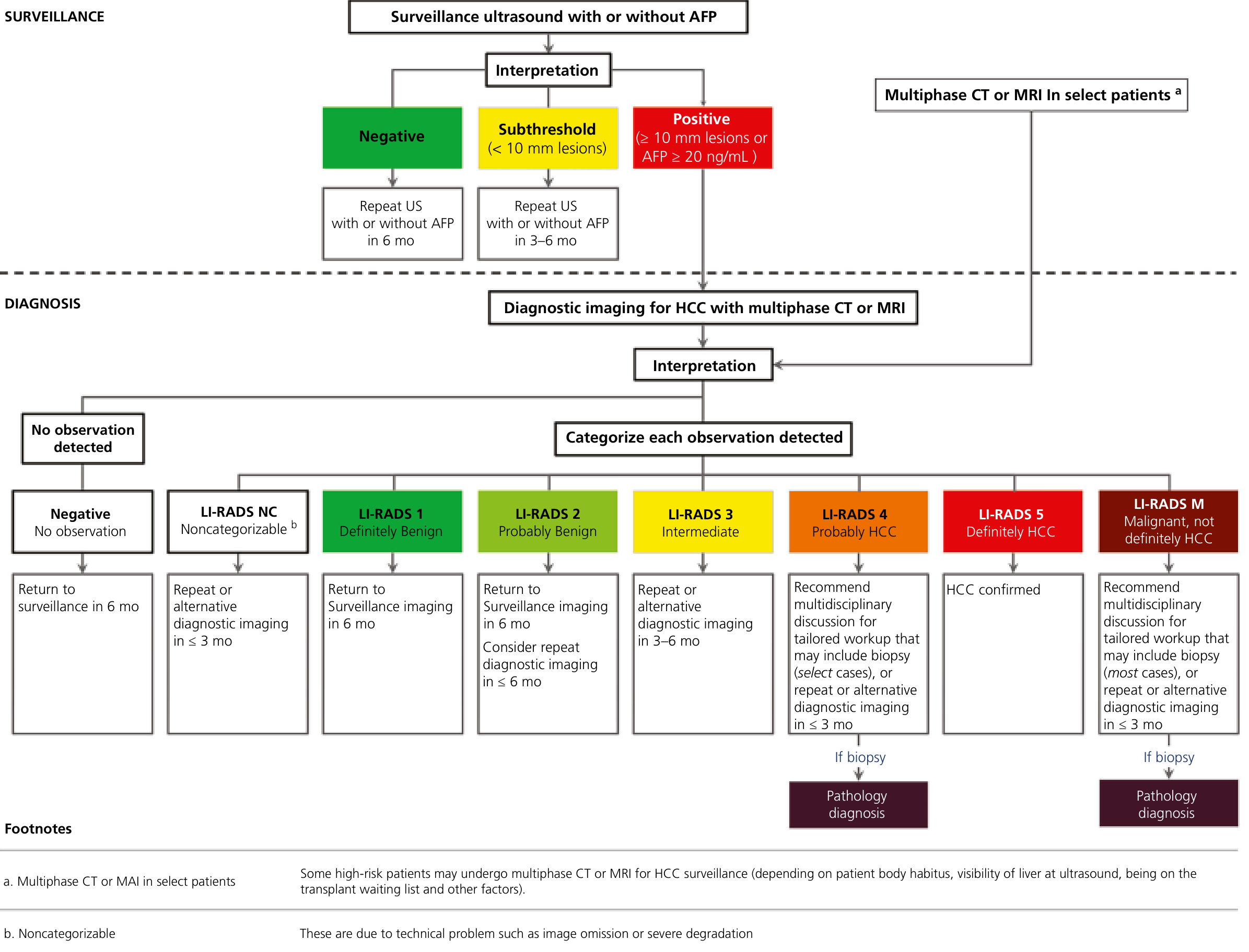
Triple-Phase CT Technique (Radiopaedia Protocol)

Patient position: Supine, arms above head
Scout: Diaphragm to iliac crests
Bolus tracking: ROI placed at aorta at level of diaphragmatic hiatus; threshold = 150 HU
Contrast: 100-120 mL non-ionic contrast at 3-5 mL/s
Scan delays:
- Late arterial: 15-30 sec post bolus trigger (35-45 sec after injection start)
- Portal venous: 60-75 sec after injection (independent of arterial timing)
- Delayed: 2-5 minutes
Respiration: Inspiration, breath-hold for each phase

CT Abdomen Contrast vs. Triple-Phase - Key Differences

Feature	Standard CT Abdomen Contrast	Triple-Phase CT
Phases acquired	Usually 1 (portal venous)	3 (arterial + portal venous + delayed)
Radiation dose	Lower	Higher (3x acquisitions)
Primary use	General abdominal pathology	Liver/pancreatic lesion characterization
Lesion detection	Good for most pathology	Optimized for focal liver lesions, HCC, hypervascular tumors
Cost and time	Lower	Higher

Radiation Considerations

Triple-phase CT delivers significantly higher radiation due to multiple acquisitions. According to research on dose reduction strategies, the unenhanced phase can be acquired at 3-fold reduced tube current without affecting attenuation value measurements, achieving a 22% total dose reduction while maintaining diagnostic quality in the contrast-enhanced phases.

Key principles for dose reduction in CT abdomen:

Use automatic exposure control (AEC)
Reduce dose on non-contrast phase (lower image quality acceptable)
In children: split-bolus technique to achieve both arterial and venous enhancement in a single acquisition (Grainger & Allison's)
Avoid triple-phase unless specifically clinically indicated

Summary of Clinical Use

Clinical Question	Recommended CT Protocol
Acute abdominal pain (appendicitis, diverticulitis)	CT abdomen/pelvis with IV contrast (portal venous phase)
Abdominal trauma	Non-contrast + arterial + portal venous (3-phase)
GI bleeding	Non-contrast + arterial + portal venous
Liver mass / HCC screening positive	Triple-phase CT (arterial + portal venous + delayed)
Colorectal liver mets staging	Triple-phase CT chest/abdomen/pelvis
Pancreatic mass	Pancreatic protocol CT (pancreatic phase ~45s + portal venous)
Renal mass	CT renal mass / washout protocol
Mesenteric ischemia	CT angiography (arterial + portal venous phases)

Give me the protocol for CT Carotid ANGIO

CT Carotid Angiography (CTA Neck/Carotids) evaluates the carotid and vertebral arteries from the aortic arch to the circle of Willis. It requires precise arterial phase timing to capture peak contrast in the carotid system.

Searching sources...

Finding Sources

Searching the Web

CT carotid angiography protocol technique scan parameters contrast timing CTA neck

Finding Sources

Reading Web Page

https://www.asnr.org/wp-content/uploads/2017/01/5_Cervicocer…

Finding Sources

Searching the Web

CTA carotid protocol radiopaedia scan range kVp mAs slice thickness bolus tracking

Reading File

Loading Image

Here is the complete CT Carotid Angiography (CTA Neck) protocol, compiled from ACR-ASNR guidelines, major radiology textbooks, and institutional protocols:

CT Carotid Angiography (CTA Neck) Protocol

Indications

Clinical Scenario	Detail
Carotid artery stenosis	TIA, ischemic stroke, amaurosis fugax
Carotid artery dissection	Spontaneous or post-trauma
Pre-operative planning	Before carotid endarterectomy (CEA) or carotid artery stenting (CAS)
Stroke workup	To assess extracranial and intracranial vessels
Aortic arch anatomy	Variant anatomy, subclavian steal, innominate artery disease
Carotid body tumor / vascular mass	Characterization
Post-procedural follow-up	Post-stent, post-CEA surveillance
Vertebrobasilar insufficiency	Vertebral artery origin stenosis

CTA has an overall sensitivity of 97% and specificity of 99% for detecting carotid stenosis. - Fischer's Mastery of Surgery

Patient Preparation

Step	Detail
IV access	20G or larger antecubital catheter - preferably RIGHT arm (avoids streak artifact from undiluted contrast in the left brachiocephalic vein)
Saline flush test	Test the line with a rapid saline bolus before contrast injection to confirm patency
Renal function screening	Check creatinine/eGFR before contrast
Allergy history	Document iodine contrast allergy; premedicate if needed
Hydration	Adequate IV hydration, especially in CKD patients
Patient positioning	Supine, arms along the chest/sides (not above head, as shoulder elevation can degrade neck vessel visualization)
Breath hold / respiration	Free breathing / quiet breathing - no breath hold needed (unlike chest CT); swallowing should be avoided during scan

Right arm injection is preferred per ACR-ASNR guidelines to prevent artifact from undiluted contrast pooling in the left brachiocephalic vein overlying the arch vessels.

Scout / Topogram

AP and lateral scout
Coverage from thorax through vertex of skull
Used to plan scan range

Scan Parameters

Parameter	Value
Scan mode	Helical (mandatory for CTA)
Gantry rotation time	≤0.5 sec per rotation
kVp	100-120 kVp (lower kVp increases contrast enhancement; use 100 kVp in average-sized patients to reduce dose and boost iodine signal)
mAs	180 mAs (AEC preferred - automatic exposure control)
Detector collimation	0.75 mm (16-slice) to 0.5 mm (64-slice and above)
Slice thickness (acquisition)	≤1.5 mm (ACR-ASNR guideline); most institutions use 0.75-1.25 mm
Reconstruction interval	≤50% of slice thickness (i.e., overlapping reconstructions - e.g., 1 mm slices at 0.5 mm increments)
Reconstruction kernel	Soft tissue / standard (NOT bone kernel - too noisy for vessels)
Pitch	~0.8-1.0 (fast pitch appropriate for CTA to minimize scan time)
FOV	250-350 mm (adjust to patient)

Scan Coverage

Boundary	Coverage
Inferior extent	Aortic arch / origin of great vessels (below aortic arch)
Superior extent	Vertex of skull / mid-orbits (2 cm above sella turcica)

Full coverage includes:

Aortic arch and origin of subclavian/brachiocephalic arteries
Common carotid arteries
Carotid bifurcation (most important area)
Internal and external carotid arteries (cervical course)
Vertebral arteries (origin to skull base)
Circle of Willis and intracranial vessels
Up to vertex

"CTA and CEMRA both allow a full assessment of the arterial tree from the aortic arch to the circle of Willis and beyond." - Grainger & Allison's Diagnostic Radiology

Scan Direction

Craniocaudal (head to foot) is inferior to superior - IMPORTANT:

Scan direction should be inferior to superior (craniocaudal approach going from aortic arch upward)
This follows the direction of contrast flow from heart → carotid arteries → brain
Scanning in the direction of blood flow ensures contrast is present in each vessel segment as the scanner reaches it
Some institutions use craniocaudal (top to bottom) to reduce perivenous streak artifact from contrast in the subclavian/brachiocephalic vein - this is an alternative validated approach

Contrast Protocol

Parameter	Value
Contrast agent	Non-ionic iso-osmolar or low-osmolar iodinated contrast (e.g., Omnipaque 350, Isovue 370, Iohexol)
Volume (adult)	80-135 mL (institutions vary: OHSU uses 50 mL at high flow; most protocols use 80-120 mL; ACR minimum 4 mL/sec in patients ≥50 kg)
Injection rate	4-5 mL/sec minimum (up to 6 mL/sec in larger patients); higher flow rate = sharper bolus = better arterial enhancement
Saline chaser	30-50 mL saline flush at same rate immediately after contrast - reduces total contrast volume needed and pushes contrast bolus through venous system
Pediatric dosing	Weight-based; scale injection rate proportionally; use right arm access

Bolus Timing - Bolus Tracking (Preferred Method)

Automatic triggering (SmartPrep / CARE Bolus / Sure-Start) is the standard:

Place ROI (region of interest) in the ascending aorta or aortic arch
Run low-dose monitoring scans every 1 second starting 5 seconds after contrast injection begins (monitoring at 100 kVp, 20-40 mAs)
Trigger threshold: 100-150 HU above baseline in the aorta
When threshold is reached, scanner automatically initiates the CTA acquisition (with a typical 5-8 second delay for table/gantry prep + patient instruction)

Alternative - Test Bolus:

Inject 10-15 mL test bolus at same flow rate
Serial low-dose scans at the aortic arch level every 1-2 seconds
Measure time to peak enhancement → use as fixed scan delay for full bolus

Pre-Contrast Phase

A non-contrast series may be obtained first when:

Suspected mural hemorrhage (dissection - intramural hematoma appears bright pre-contrast)
Mapping calcification for stenosis assessment
Localizing anatomy

Section thickness for non-contrast: same as CTA or ≤5 mm (ACR-ASNR).

Reconstructions / Post-Processing

After raw acquisition, the following reformats are generated:

Reconstruction	Detail
Axial source images	1 mm thickness, reviewed first - most important for stenosis measurement
Sagittal reformats	1 mm
Coronal reformats	1 mm
Sagittal MIP (Maximum Intensity Projection)	3 mm slabs - shows vessel course and stenosis
Coronal MIP	3 mm slabs
3D Volume Rendering (VR)	Overall vascular anatomy, surgical planning, patient communication
Curved planar reformations (CPR)	Straightens vessel for accurate stenosis length measurement
Bone subtraction	Software removes skull base/cervical spine to better visualize vessels

Window settings for viewing: W400/L40 (standard soft tissue) for axial; adjust to W730/L310 for heavily calcified stenoses.

What the Radiologist Reports

Degree of stenosis using NASCET criteria:
- Stenosis % = (1 - residual lumen diameter / normal distal ICA diameter) × 100
- Symptomatic: ≥70% stenosis = high benefit from CEA; 50-69% = moderate benefit
Plaque morphology (calcified vs. soft/lipid-rich - juxtoluminal hypodensity = unstable plaque)
Occlusion vs. near-occlusion ("trickle flow")
Tandem lesions (intracranial + extracranial disease)
Carotid bulb/ICA anatomy, tortuosity, kinks, coils
Aortic arch type and variant origin of vessels (surgical planning)
Vertebral artery dominance/patency
Circle of Willis completeness

CTA vs. Other Modalities for Carotid Stenosis

Modality	Sensitivity	Specificity	Key Notes
CTA	97%	99%	No flow artifacts; shows calcification well; radiation + contrast
Duplex US	~90%	~90%	First-line, operator-dependent; cannot assess arch
CE-MRA	94%	93%	No radiation; may overestimate stenosis; can miss calcification
DSA (catheter)	Gold standard	Gold standard	Invasive; 1% stroke risk; required before carotid stenting

Fischer's Mastery of Surgery, Grainger & Allison's Diagnostic Radiology

Example CTA Carotid Image

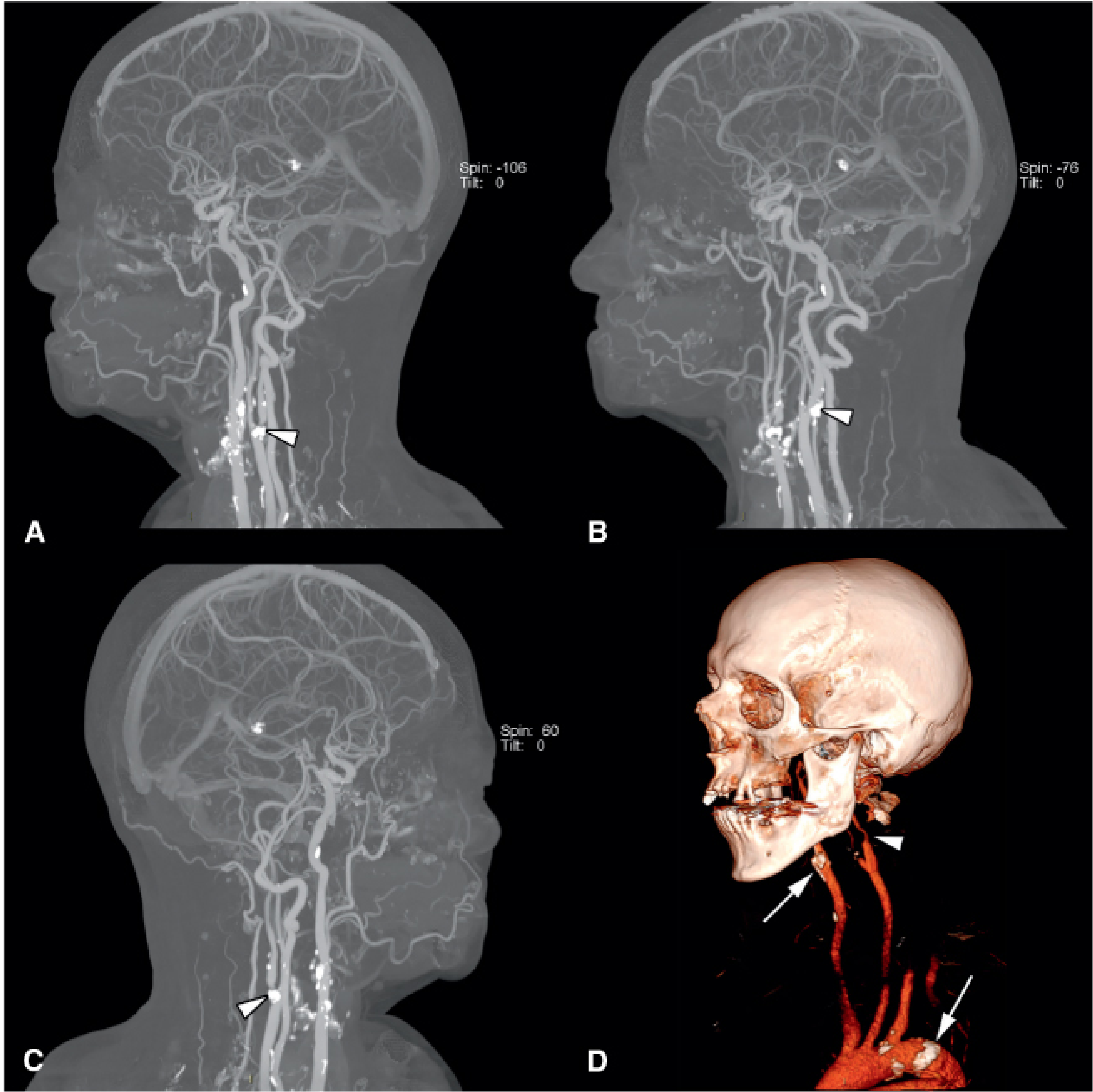
CT angiogram of carotid and vertebral arteries showing 3D reconstructions with area of approximately 90% stenosis of the left internal carotid artery

CTA head and neck with 3D vessel reconstruction. Arrowheads show carotid bifurcation calcification; the right image (D) shows a 3D bone-subtracted volume rendering with approximately 90% stenosis of the left ICA. - Fischer's Mastery of Surgery

Key Tips and Pitfalls

Issue	Solution
Venous contamination (left brachiocephalic vein streak)	Use right arm injection; consider craniocaudal scan direction
Heavy calcification	Adjust window width; use CTA source images (not MIP) to measure true lumen
Arterial-venous overlap	Optimize timing with bolus tracking; avoid late acquisition
Motion artifact (swallowing)	Instruct patient not to swallow during scan; short scan time helps
Contrast nephropathy	Screen creatinine; hydrate; use minimum effective contrast volume
Near-occlusion	CTA source images + MIP together; arterial + slightly delayed phase discriminate occlusion from trickle flow

Explain me clearly SNR , CNR & Bandwidth

These are core imaging physics concepts relevant to both MRI and CT. Let me give you a thorough explanation while pulling from the textbooks.

Searching sources...

Finding Sources

Searching Images

SNR CNR signal to noise ratio contrast to noise ratio MRI imaging diagram

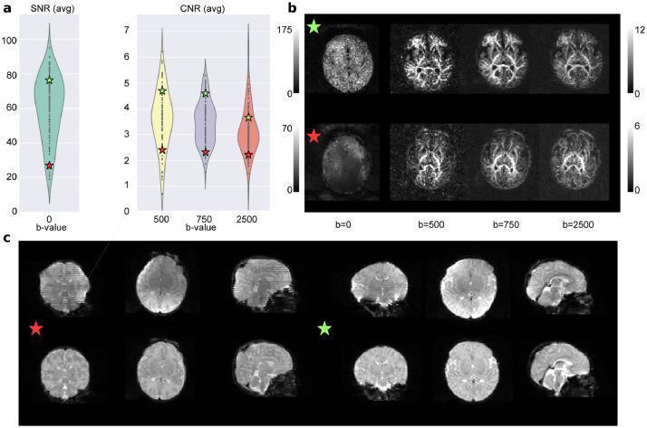
This three-panel figure illustrates quality control (QC) metrics for neonatal diffusion MRI (dMRI) data processing. Panel (a) features violin plots displaying the distribution of average Signal-to-Noise Ratio (SNR) at b=0 and Contrast-to-Noise Ratio (CNR) at b-values of 500, 750, and 2500 s/mm² for the study population. Two representative subjects are highlighted: a high-quality outlier (green star) and a low-quality outlier (red star). Panel (b) presents the corresponding axial SNR and CNR maps for these two subjects, demonstrating superior signal intensity and structural definition in the high-SNR subject across all b-values, while the low-SNR subject exhibits significant noise and reduced contrast. Panel (c) compares b0 intensity images for both subjects before (top row) and after (bottom row) a processing pipeline. The comparison highlights the pipeline's efficacy in correcting Echo Planar Imaging (EPI) geometric distortions and magnetic field inhomogeneities. For the red-star subject, the post-processing images show marked reduction in signal dropout and improved anatomical alignment, illustrating the importance of rigorous QC in neonatal neuroimaging research.

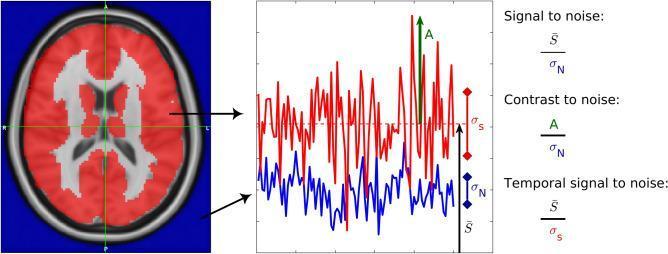
This infographic illustrates functional Magnetic Resonance Imaging (fMRI) quality metrics, combining an axial diagnostic brain image with a signal processing plot. On the left, an axial MRI slice highlights specific regions in red, indicating brain activity areas compared to background tissue. Arrows map these areas to a central time-series plot. The plot features two waveforms: a red signal representing brain activity and a blue signal representing background noise. Key mathematical parameters are annotated: 'S-bar' (horizontal dashed line) represents the mean brain activity signal; 'sigma_S' and 'sigma_N' denote the standard deviations of the brain activity and background noise, respectively; and 'A' (green arrow) indicates the maximum peak amplitude of the brain activity. On the right, three critical quality metric formulas are defined: Signal-to-Noise Ratio (SNR) as S-bar/sigma_N, Contrast-to-Noise Ratio (CNR) as A/sigma_N, and Temporal Signal-to-Noise Ratio (tSNR) as S-bar/sigma_S. This educational diagram is designed for neurology and radiology students to understand the quantitative assessment of signal quality in neuroimaging.

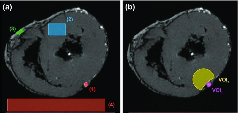
Diagnostic Magnetic Resonance Imaging (MRI) cross-sections of an ex vivo heart demonstrating quantitative analysis methods. Image (a) depicts a morphological T1-weighted scan with four labeled Regions of Interest (ROI) used for calculating signal-to-noise ratio (SNR) and contrast-to-noise ratio (CNR): ROI 1 (red square) targets the hyperintense perfusate in a vessel; ROI 2 (blue rectangle) is positioned within the mid-myocardium; ROI 3 (green rectangle) covers the epicardial fat; and ROI 4 (large red rectangle) is placed in the background to measure image noise. Image (b) shows Volumes of Interest (VOI) focused on the anterior wall: VOI 1 (violet circle) identifies the Left Anterior Descending (LAD) artery filled with contrast agent, and VOI 2 (yellow crescent) identifies the adjacent myocardium. The images serve as an educational example of how different tissue compartments (perfusate, muscle, and fat) are segmented to evaluate imaging sequences and perfusate efficacy in cardiovascular research. For orientation, the anterior cardiac wall is positioned at the bottom of the frames.

The library doesn't have a dedicated MRI physics textbook, so I'll synthesize a thorough explanation from first principles, supplemented by what the textbooks do say. Here is a complete, structured explanation:

SNR, CNR & Bandwidth in Medical Imaging

1. SNR - Signal-to-Noise Ratio

What is it?

SNR is the most fundamental measure of image quality. It tells you how much useful signal you have compared to the background noise.

$$\boxed{SNR = \frac{\text{Signal (mean intensity in tissue)}}{\text{Noise (SD of background)}}}$$

Signal = the average pixel/voxel intensity coming from the tissue of interest
Noise = random fluctuations in pixel intensity that don't carry any useful information (measured as standard deviation in a background air region)

Simple analogy

Think of trying to hear someone talk at a party. The person's voice = signal. The background chatter = noise. A high SNR means you can hear them clearly. A low SNR means they're drowned out.

In MRI

In MRI, signal comes from protons in tissue precessing and emitting radiofrequency energy. Noise comes from:

Thermal noise from the patient's body (dominant source)
Electronic noise from the receiver coil and circuitry
External electromagnetic interference

Factors that INCREASE SNR in MRI

Factor	Effect	Why
Higher field strength (B0)	↑↑ SNR	More protons align; signal proportional to B0²
Larger voxel size	↑ SNR	More protons per voxel = more signal
Thicker slice	↑ SNR	More protons in the volume
More signal averages (NSA/NEX)	↑ SNR	SNR ∝ √NSA (doubling NSA gives √2 ≈ 1.41× SNR)
Smaller receiver bandwidth	↑ SNR	Less noise sampled (explained below)
Surface coils / array coils	↑ SNR	Coil closer to tissue = better coupling
Longer TR	↑ SNR (T1-weighted)	More longitudinal magnetization recovery
Shorter TE	↑ SNR	Less T2 decay before readout

Factors that DECREASE SNR

Factor	Effect
Smaller voxel (higher resolution matrix)	↓ SNR
Thinner slices	↓ SNR
Lower field strength magnet	↓ SNR
Larger bandwidth	↓ SNR
Shorter TR or longer TE	↓ SNR (in many sequences)

The fundamental SNR trade-off

Higher spatial resolution = smaller voxels = LOWER SNR

You can't have perfect resolution AND perfect SNR simultaneously. You always trade one for the other. This is one of the central challenges of MRI protocol design.

SNR formula for MRI:

$$SNR \propto \text{Voxel Volume} \times \sqrt{N_{ex}} \times \sqrt{N_{PE}} \times \frac{1}{\sqrt{BW}}$$

Where:

Voxel Volume = FOV²/matrix² × slice thickness
NEX = number of excitations (averages)
NPE = number of phase encoding steps
BW = receiver bandwidth

2. CNR - Contrast-to-Noise Ratio

What is it?

CNR measures the ability to distinguish two adjacent tissues from each other relative to background noise.

$$\boxed{CNR = \frac{|Signal_A - Signal_B|}{Noise}}$$

Signal_A = mean intensity of tissue A (e.g., grey matter)
Signal_B = mean intensity of tissue B (e.g., white matter)
Noise = SD of background

Why CNR matters MORE than SNR for diagnosis

You can have a very high SNR image (low noise, bright signal) but still not be able to distinguish a liver metastasis from normal liver if they have identical signal intensities. CNR determines diagnostic usefulness.

SNR tells you how clear the image is. CNR tells you whether you can actually see pathology.

Visual explanation

fMRI quality metrics diagram showing SNR as mean signal / noise SD, and CNR as peak amplitude / noise SD

SNR = mean brain signal / noise SD; CNR = peak amplitude (contrast) / noise SD

Factors that affect CNR

CNR depends on both SNR and image contrast:

$$CNR = Contrast \times SNR$$

So to improve CNR, you can either:

Increase SNR (all the methods above), OR
Increase contrast between tissues (sequence/parameter selection)

How contrast is created in MRI

Sequence weighting	What creates contrast	High signal vs low signal
T1-weighted	T1 relaxation differences	Fat bright, fluid dark
T2-weighted	T2 relaxation differences	Fluid bright, fat intermediate
PD-weighted	Proton density differences	Tissues with many protons bright
Gadolinium contrast	T1 shortening in enhancing tissue	Enhancing lesion bright vs non-enhancing dark
DWI	Diffusion restriction	Restricted diffusion bright

CNR in CT

In CT, CNR is determined by:

HU difference between tissues (inherent contrast)
Image noise (↓ with higher mAs, larger slice, lower pitch)
Iodinated contrast (increases HU difference between vessels/lesions and background)

Key CT CNR example: A liver metastasis at 45 HU in a liver at 60 HU = only 15 HU difference. Without contrast, CNR is poor. With contrast (portal venous phase), the liver enhances to 100+ HU while a hypovascular met stays at 45 HU → difference = 55+ HU → CNR greatly improved → lesion now visible.

CNR in MRI: measuring it

MRI cross-sections showing ROI placement for SNR and CNR measurement - tissue ROIs and background noise ROI

Practical CNR measurement: ROI 1 in tissue A (vessel), ROI 2 in tissue B (myocardium), ROI 4 in background air for noise measurement. CNR = |mean ROI1 - mean ROI2| / SD(ROI4)

3. Bandwidth

Bandwidth is one of the most misunderstood but important parameters in MRI. There are actually two types - receive bandwidth and transmit bandwidth.

A. Receive Bandwidth (Readout Bandwidth / Frequency Bandwidth)

This is the bandwidth you control on the scanner console. It refers to the range of radiofrequencies sampled during the frequency-encoding (readout) gradient.

The physics behind it

During frequency encoding in MRI:

A readout gradient is applied across the patient
Protons at different positions along this gradient precess at different frequencies (Larmor frequency varies with position)
The receiver coil "listens" to a range of frequencies - this range is the receiver bandwidth

Units: Hz/pixel or kHz total (e.g., ±16 kHz means 32 kHz total bandwidth)

Bandwidth and Noise - the critical relationship

$$\text{Noise} \propto \sqrt{BW}$$ $$SNR \propto \frac{1}{\sqrt{BW}}$$

Why? The receiver amplifies everything it can "hear" - including noise. A wider bandwidth means the receiver is tuned to a wider frequency range, so it picks up more thermal/electronic noise.

Narrow bandwidth = receiver listens to a narrow range of frequencies = less noise = higher SNR
Wide bandwidth = receiver listens to a broad range = more noise = lower SNR

Bandwidth and Sampling Time

$$BW = \frac{1}{\Delta t} \quad \text{(inversely related to dwell time per sample)}$$

Narrow bandwidth → longer sampling time per frequency line → longer echo spacing → longer minimum TE
Wide bandwidth → shorter sampling time → shorter minimum TE

Key effects of changing bandwidth

Effect	Narrow BW (e.g., ±8 kHz)	Wide BW (e.g., ±32 kHz)
SNR	↑ Higher	↓ Lower
Minimum TE	↑ Longer (must wait longer to sample)	↓ Shorter
Chemical shift artifact	↑ MORE artifact	↓ Less artifact
Scan time	Longer (each readout takes more time)	Shorter
Geometric distortion (EPI)	More	Less

Chemical Shift Artifact and Bandwidth - KEY EXAM POINT

Chemical shift artifact occurs at fat-water interfaces (e.g., kidney edge, orbit) because fat protons precess ~3.5 ppm slower than water protons.

$$\text{Chemical shift (pixels)} = \frac{\Delta f_{fat-water}}{BW_{per pixel}}$$

Narrow bandwidth = each pixel represents a smaller frequency range → fat and water pixels are displaced MORE pixels apart → MORE chemical shift artifact
Wide bandwidth = each pixel covers a larger frequency range → fat/water shift spans fewer pixels → LESS chemical shift artifact

Trade-off summary:

Narrow bandwidth → better SNR but more chemical shift artifact and longer TE Wide bandwidth → worse SNR but less chemical shift artifact and shorter TE

B. Transmit Bandwidth (RF Pulse Bandwidth)

This is a different concept - it's the range of frequencies in the excitation RF pulse used to excite a slice.

$$\text{Slice thickness} = \frac{BW_{transmit}}{G_{slice}}$$

Where G_slice = slice selection gradient strength.

A wider transmit bandwidth with the same gradient = thicker slice
A narrower transmit bandwidth with the same gradient = thinner slice
Alternatively, keeping the same bandwidth but increasing the gradient = thinner slice

This is how the scanner controls slice thickness without changing anything visible to the operator.

4. The Interrelationships - The Big Picture

These three parameters are deeply connected. Every MRI protocol is a set of compromises:

HIGH SNR ←→ LARGE VOXEL (low resolution)
HIGH CNR ←→ OPTIMAL SEQUENCE WEIGHTING + HIGH SNR
HIGH SNR ←→ NARROW BANDWIDTH (but more chemical shift + longer TE)
HIGH SNR ←→ MORE AVERAGES (but longer scan time)

The SNR/CNR/Bandwidth Triangle in Practice

If you want to...	Do this	But accept...
Better SNR	Increase voxel size (thicker slice, larger FOV, coarser matrix)	Lower spatial resolution
Better SNR	Add more averages (NEX)	Longer scan time
Better SNR	Narrow the bandwidth	More chemical shift artifact; longer TE
Better CNR	Choose the right sequence weighting (T1/T2/T2*)	Sequence-specific
Better CNR	Give contrast agent (Gad)	Cost, nephrogenic risk
Less chemical shift artifact	Widen the bandwidth	Lower SNR
Shorter TE	Widen the bandwidth	Lower SNR

5. Quick Summary Table

Parameter	Formula	What it measures	Key determinants
SNR	Mean signal / Noise SD	Overall image clarity	Voxel size, B0, coil, bandwidth, averages
CNR	\|Signal_A - Signal_B\| / Noise SD	Ability to distinguish two tissues	SNR × tissue contrast
Receive BW	Range of frequencies sampled (Hz/pixel)	Noise sampled; TE flexibility; chemical shift	↑BW = ↓SNR, ↓artifact, ↓TE
Transmit BW	Frequency range of RF pulse (Hz)	Slice thickness selection	↑BW with same gradient = thicker slice

6. Clinical Scenario Examples

Scenario 1: You're imaging a small internal auditory canal lesion (acoustic neuroma). You need high spatial resolution.

Small voxels needed → SNR drops → compensate by: narrowing bandwidth (↑SNR but watch for chemical shift), adding averages, using surface coil, using 3T instead of 1.5T.

Scenario 2: You see fat-water chemical shift artifact around the kidney on a T1 image.

Increase receiver bandwidth → artifact decreases → accept slight SNR penalty.

Scenario 3: A liver lesion is barely visible on unenhanced MRI.

SNR may be adequate but CNR is low (lesion and liver have similar signal)
Give gadolinium → enhances lesion → increases signal difference → improves CNR → lesion now detectable.

Scenario 4: Patient can't hold breath and motion artifact is present.

Increase bandwidth → shorter TE, faster readout → less time for motion during each acquisition → reduces motion blurring (at cost of some SNR).

Explain me in detail about MRI Sequences - CISS, FLAIR, STIR, T2, T1 and their uses

These are the backbone sequences of clinical MRI. Let me pull detailed content from the radiology textbooks.

Searching sources...

Finding Sources

Reading File

Finding Sources

Reading File

Finding Sources

Searching Images

MRI sequences T1 T2 FLAIR STIR brain comparison

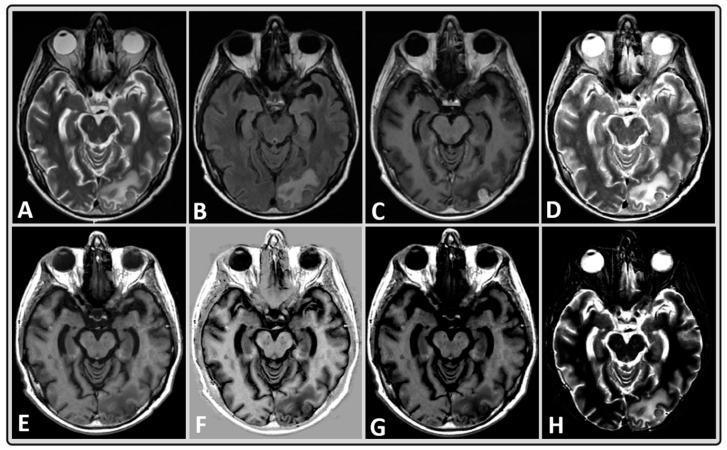
A comparison panel of axial brain MRI sequences from a 40-year-old male with brain metastasis. The top row (A-C) shows standard clinical acquisitions: (A) T2-weighted (T2w), (B) T2-weighted Fluid Attenuated Inversion Recovery (FLAIR), and (C) T1-weighted (T1w) post-contrast. The remaining images (D-H) are synthetically generated (MAGiC): (D) T2w, (E) T1w, (F) Phase-Sensitive Inversion Recovery (PSIR), (G) T1w FLAIR, and (H) Short Tau Inversion Recovery (STIR). The images demonstrate a focal lesion in the left occipital region, which appears hyperintense on T2w and FLAIR sequences and shows significant enhancement on the post-contrast T1w image (C). The synthetic images (D-H) replicate key tissue contrasts, such as bright CSF in T2w (D) and STIR (H), suppressed CSF signal in FLAIR (B, G), and the characteristic gray-white matter differentiation of T1w (E) and PSIR (F). This clinical image set illustrates the utility of synthetic MRI in obtaining multiple diagnostic weightings from a single rapid acquisition.

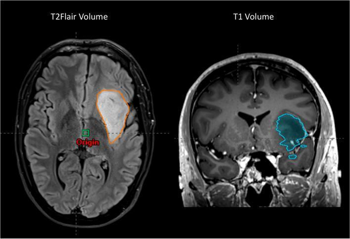
This diagnostic image displays a side-by-side comparison of two MRI sequences—T2 FLAIR (axial view, left) and T1-weighted (coronal view, right)—demonstrating the methodology for tumor volume measurement in a patient with a brain tumor, likely a glioma. In the T2 FLAIR image, the lesion appears hyperintense (bright) and is outlined by an orange contour, highlighting the total extent of the tumor and associated vasogenic edema or infiltrative disease. In the T1-weighted image, the corresponding tumor volume is hypointense (dark) and outlined with a blue contour. Both images feature anatomical orientation markers and an 'Origin' point for spatial normalization, typically used in radiation therapy treatment planning. The visual emphasizes the different signal characteristics of brain pathology across modalities: T2 FLAIR is highly sensitive to tissue water content and edema, while T1 provides superior anatomical detail and shows the core lesion as a low-signal area. This comparison is clinically relevant for neuro-oncology trainees and neuroradiologists for accurate lesion delineation and longitudinal monitoring of tumor response.

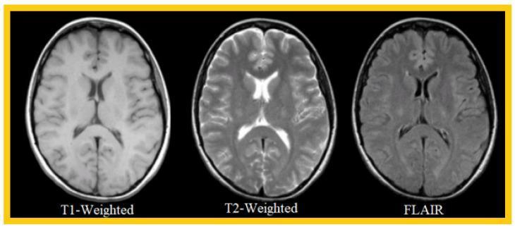
This diagnostic image provides a side-by-side comparison of three common Magnetic Resonance Imaging (MRI) sequences in the axial plane of the human brain: T1-weighted, T2-weighted, and Fluid-Attenuated Inversion Recovery (FLAIR). The comparison illustrates the varying signal intensities of intracranial tissues and fluids across modalities. In the T1-weighted image, cerebrospinal fluid (CSF) is hypointense (dark), while white matter appears hyperintense (bright) relative to gray matter, highlighting excellent anatomical detail and cortical architecture. The T2-weighted sequence shows CSF as hyperintense (bright) and white matter as hypointense, effectively demonstrating fluid-containing spaces like the ventricles and sulci. The FLAIR sequence resembles T2 weighting but utilizes signal suppression to make CSF appear dark, which enhances the visibility of periventricular lesions or cortical pathology that might otherwise be obscured by bright fluid. This comparison is fundamental for medical education in neuroradiology, aiding in the identification of normal anatomy and the selection of appropriate sequences for detecting specific brain pathologies such as tumors or edema.

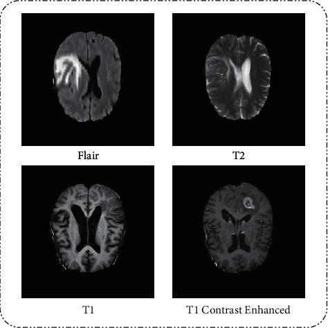
This diagnostic image provides a comparison of four axial MRI sequences of the human brain, used for neuro-oncological evaluation: FLAIR, T2-weighted, T1-weighted, and T1-weighted with contrast enhancement (T1CE). The FLAIR sequence highlights a large hyperintense (bright) region in the left cerebral hemisphere, representing vasogenic edema or non-enhancing tumor. The T2-weighted scan shows similar hyperintensity, particularly emphasizing cerebrospinal fluid and peri-ventricular changes. The native T1-weighted image provides anatomical detail with low signal intensity in the pathological regions. The T1CE image reveals a distinct, irregular ring-enhancing lesion in the right frontal/parietal area with a central hypointense core, suggestive of tumor necrosis, characteristic of high-grade glioma such as glioblastoma. This comparison illustrates how different MRI modalities allow for the differentiation of tumor core, enhancement, and surrounding edema in clinical diagnostics.

Loading Image

Finding Sources

Here is a detailed, structured explanation of all six MRI sequences - their physics, signal characteristics, and clinical uses.

MRI Sequences: T1, T2, FLAIR, STIR, CISS - Complete Guide

The Foundations: TR, TE, and TI

Before understanding the sequences, you need to know the three timing parameters that define them:

Parameter	Full Name	What it controls
TR	Repetition Time	Time between successive RF excitation pulses (controls T1 weighting)
TE	Echo Time	Time from RF pulse to signal readout (controls T2 weighting)
TI	Inversion Time	In inversion recovery sequences - time between 180° inversion pulse and 90° excitation pulse (controls what tissue signal is nulled)

1. T1-Weighted Imaging (T1WI)

Parameters

Short TR (500-700 ms) + Short TE (15-40 ms)
Spin echo or gradient echo technique

How it works

Short TR means tissues don't fully recover their longitudinal magnetization between pulses. Tissues with fast T1 relaxation (fat, gadolinium-enhanced tissue) recover faster and appear bright. Tissues with slow T1 relaxation (water/CSF) haven't recovered and appear dark.

Signal characteristics - the quick identification rule

Tissue	T1 Signal	Reason
Fat	Bright (white)	Short T1 - fast recovery
CSF / free fluid	Dark (black)	Long T1 - slow recovery
Bone marrow	Bright	Fat content
Cortical bone / air	Dark
Muscle	Intermediate grey
Most tumors/masses	Intermediate (like muscle)
Subacute hemorrhage (methemoglobin)	Very bright	Paramagnetic T1 shortening
Gadolinium-enhanced tissue	Bright	T1 shortening by Gd
Melanin	Bright	T1 shortening
Protein-rich fluid	Bright	Shortened T1

Quick rule: On T1 - fat is WHITE, CSF is BLACK

Clinical uses

Application	Why T1
Anatomy	Excellent soft tissue contrast, high SNR, best anatomical detail
Fat detection	Fat appears bright; confirm with fat-sat to make it go dark
Hemorrhage staging	Subacute bleed (methemoglobin) = bright T1
Bone marrow evaluation	Normal marrow is bright from fat; infiltration appears dark
Liver steatosis	Chemical shift T1 imaging
Post-gadolinium	Always done with T1WI - enhancing lesions become bright
Pituitary / sellar	High resolution T1 pre and post Gad
Melanoma	Melanin gives bright T1 signal

Gadolinium and T1

Gadolinium shortens T1 in tissues where it distributes (areas of blood-brain barrier breakdown, highly vascular tissue, inflammation). This makes enhancing lesions brighter on post-contrast T1WI. Fat suppression is added with post-Gad T1 in the head/neck to remove competing fat signal and improve conspicuity of enhancement. - Cummings Otolaryngology

Four MRI sequences of a parapharyngeal mass: T1WI (dark mass, dark CSF), spin density, T2WI (bright mass, bright CSF), and post-gadolinium T1WI (enhancing mass)

Cummings Otolaryngology - Common MRI pulse sequences. (A) T1WI: mass is dark, CSF is dark. (C) T2WI: mass is bright, CSF is bright. (D) Post-Gad T1WI: mass enhances.

2. T2-Weighted Imaging (T2WI)

Parameters

Long TR (2000-4000 ms) + Long TE (50-90 ms)
Usually fast spin echo (FSE/TSE) in modern practice

How it works

Long TR allows full T1 recovery for all tissues (eliminating T1 contrast). Long TE allows T2 decay to differentiate tissues. Tissues with long T2 (free water, fluid) retain signal and appear bright. Tissues with short T2 (dense fibrous tissue, cortical bone, hemosiderin) lose signal and appear dark.

Signal characteristics

Tissue	T2 Signal
CSF / free fluid / vitreous	Very bright (white)
Mucosa / airway lining	Very bright
Most pathological lesions (edema, tumor, inflammation)	Bright
Fat	Intermediate-bright on FSE T2 (bright due to J-coupling in FSE)
Muscle	Intermediate-low
Cortical bone / calcification	Dark
Hemosiderin / iron	Very dark (susceptibility)
Flowing blood (fast)	Dark (flow void)
Fibrous tissue / ligaments	Dark

Quick rule: On T2 - CSF is WHITE, muscle is GREY, pathology is usually BRIGHT

Why most pathology is bright on T2

Disease processes (infection, tumor, infarct, edema, demyelination) increase tissue water content → longer T2 → brighter signal on T2WI. This makes T2 the most sensitive sequence for detecting pathology.

Clinical uses

Application	Detail
Brain lesion detection	MS plaques, tumors, infarcts, encephalitis - all bright on T2
Spine - disc disease	Disc dehydration = dark disc (normal bright disc = water content)
Musculoskeletal - cartilage	Bright signal on T2
Liver / abdominal organs	Cyst vs solid: cyst is very bright T2
Prostate	Zonal anatomy, tumor detection (T2 low signal in peripheral zone = tumor)
Female pelvis / uterus	Zonal anatomy of uterus; endometriosis, fibroids
Hepatic hemangioma	Very bright on heavily T2-weighted images ("light bulb" sign)
Spine cord	Myelopathy, cord edema, syrinx

The T2 "light bulb" sign

Hepatic hemangiomas are very bright on heavily T2-weighted sequences - bright like a light bulb because they are filled with slowly flowing blood. This distinguishes them from metastases which are not as bright.

Three-way brain MRI comparison showing T1 (dark CSF, bright white matter), T2 (bright CSF), and FLAIR (dark CSF but bright periventricular lesions visible)

Side-by-side comparison: T1-weighted (CSF dark, good anatomy), T2-weighted (CSF bright, fluid bright), FLAIR (CSF suppressed - periventricular pathology stands out)

3. FLAIR - Fluid Attenuated Inversion Recovery

Full name

Fluid-Attenuated Inversion Recovery

Parameters

Long TR (~9000-11000 ms) + Long TE (~120-140 ms) + Long TI (~2200-2500 ms)
It is an inversion recovery T2-weighted sequence

How it works - the key concept

FLAIR is essentially a T2-weighted sequence with CSF suppressed.

An initial 180° inversion pulse flips all magnetization. Tissues recover at different rates (T1 relaxation). The TI is chosen specifically to equal 0.693 × T1(CSF) so that at the moment the 90° pulse fires, the CSF magnetization is exactly at zero → CSF produces no signal → appears dark.

Everything else behaves like T2 - pathological tissue with long T2 remains bright.

$$TI_{null} = T1_{CSF} \times \ln(2) \approx 2200-2500 \text{ ms}$$

Signal characteristics

Tissue	FLAIR Signal
CSF	Dark (suppressed) - KEY feature
Free fluid	Dark (suppressed)
Normal brain parenchyma	Grey
White matter lesions (MS, infarct, gliosis)	Bright - stands out against dark CSF
Periventricular lesions	Very conspicuous - can't be hidden by adjacent bright CSF
Cortical/subcortical lesions	Highlighted against dark sulcal CSF
Subarachnoid hemorrhage (acute)	Bright (blood in subarachnoid space = bright on FLAIR)

Why FLAIR is so useful - the critical clinical insight

On standard T2WI, CSF and periventricular lesions are both bright → lesions adjacent to ventricles are invisible (hidden by surrounding bright CSF). FLAIR suppresses the CSF → lesions now stand out brilliantly against the dark background.

Clinical uses

Application	Why FLAIR
Multiple sclerosis (MS)	Periventricular plaques are hallmark - only visible on FLAIR, invisible on standard T2
Acute ischemic stroke (DWI+FLAIR mismatch)	FLAIR-negative/DWI-positive = stroke onset <4.5 hours (tissue still salvageable for thrombolysis)
Subarachnoid hemorrhage	Bloody CSF is bright on FLAIR - sensitive when CT is negative
Meningitis / meningeal disease	Meningeal enhancement/exudate visible on FLAIR
Cerebral cortical lesions	Cortical lesions highlighted against dark sulcal CSF
White matter diseases	Leukoaraiosis, CADASIL, vasculitis, metastases
Limbic encephalitis	Mesial temporal lobe FLAIR hyperintensity
Tumors	Non-enhancing tumor and edema well seen on FLAIR

Per Rosen's Emergency Medicine: DWI-positive + FLAIR-negative = acute stroke window. When FLAIR is already positive in the same region as the DWI lesion, stroke onset was likely >4.5-6 hours.

Per Harrison's Principles: Chronic lacunar infarcts on FLAIR appear as a hyperintense rim surrounding a hypointense cavitated core.

Brain MRI showing FLAIR (left, bright lesion periventricular) and T1 post-contrast (right, enhancing lesion) for tumor volume measurement and comparison

FLAIR shows total tumor extent including edema (bright); T1 post-contrast shows actively enhancing tumor core. Both are needed for complete tumor characterization.

4. STIR - Short Tau Inversion Recovery

Full name

Short Tau Inversion Recovery

Parameters

Long TR + Long TE + Short TI (120-180 ms at 1.5T)
Inversion recovery sequence

How it works

Like FLAIR, an initial 180° inversion pulse is applied. But now the TI is set short to null the signal of fat (not CSF):

$$TI_{null(fat)} = T1_{fat} \times \ln(2) \approx 140-160 \text{ ms at 1.5T}$$

At this short TI, fat magnetization is exactly at zero → fat produces no signal → fat appears completely black.

The sequence is then T2-weighted, so pathological tissue (edema, infection, tumor) with long T2 remains very bright, now without any competing fat signal.

Signal characteristics

Tissue	STIR Signal
Fat	Black (completely suppressed) - KEY feature
CSF / free fluid	Very bright
Muscle	Intermediate
Edema / inflammation	Very bright - highly conspicuous
Bone marrow edema	Very bright against nulled marrow fat
Tumors	Bright
Nerve roots	Intermediate to bright

Quick rule: On STIR - fat is BLACK, CSF and edema are WHITE

STIR vs. Frequency-Selective Fat Saturation

Feature	STIR	Chemical Shift Fat Sat
Fat suppression	By T1 nulling (reliable)	By frequency selection
Field homogeneity requirement	Robust - works at any field	Requires homogeneous B0
Body parts with curved surfaces	Works well	Fails at edges/extremities
Cannot use with Gadolinium	True - Gad also shortens T1 of other tissues, may inadvertently suppress enhancing lesions	Gad-compatible
SNR	Lower	Higher
Scan time	Longer	Faster

STIR's major advantage: it works reliably even with inhomogeneous magnetic fields (at extremities, large body parts, air-tissue interfaces) where chemical shift fat saturation fails. - Cummings Otolaryngology

Clinical uses

Application	Detail
Bone marrow edema	Stress fractures, osteomyelitis, bone metastases, trauma - marrow edema brilliant on STIR
Spine - ligament injury	Cervical spine trauma, cord edema, ligamentous injury
Perianal fistula	Fistula tracts appear very bright against dark fat
Muscle edema/myositis	Inflammatory myopathies - edema bright against black fat
Brachial/lumbosacral plexus	Nerve root/plexus edema and pathology
Whole body MRI	Screening for bone mets (STIR preferred for whole body)
Soft tissue tumors	Excellent for delineating extent against fat background
Acute pyelonephritis	Gadolinium-enhanced STIR for renal inflammation
Extremity imaging	Preferred fat suppression at hands, feet, ankles where fat sat fails

Per Grainger & Allison's: Spine MRI standard protocol includes sagittal T1, sagittal T2, sagittal T2 with STIR (fat suppression), and axial T2.

Per Rheumatology textbook: "Adding fat suppression to T2 in the form of STIR sequences improves detection of muscle inflammation by enhancing the bright signal of edema and decreasing the fat signal."

5. CISS - Constructive Interference in Steady State

Full name

Constructive Interference in Steady State (Siemens terminology; equivalent sequences: FIESTA on GE, BFFE on Philips, True-FISP variants)

Sequence type

A heavily T2-weighted 3D gradient echo (steady-state free precession - SSFP) sequence

Parameters

Very short TR (typically 5-20 ms) and short TE
Flip angle ~70°
The key: it acquires images in steady state with very thin slices (0.4-0.8 mm)

How it works

Unlike spin echo sequences, CISS is a gradient echo steady-state sequence. It produces extremely high contrast between fluid (very bright) and soft tissue/nerves (dark). Because the TR is very short, both T1 and T2 contribute, but the net effect is very high T2/T1 ratio - fluid is extremely bright.

The "constructive interference" refers to combining two phase-cycled acquisitions to eliminate banding artifacts from field inhomogeneity that normally plague SSFP sequences.

Signal characteristics

Tissue	CISS Signal
CSF / fluid	Extremely bright (white)
Cranial nerves	Dark (well-defined) against bright CSF
Vessels	Dark flow void
Bone	Dark
Soft tissue	Intermediate-dark
Fat	Intermediate

The defining feature

CISS achieves sub-millimeter isotropic resolution with very high contrast between CSF and soft tissue structures. This allows visualization of tiny structures floating in CSF (cranial nerves, the VIII nerve, cochlear structures, inner ear anatomy).

Clinical uses

Application	Why CISS
Inner ear / cochlea imaging	Gold standard - shows cochlear turns, semicircular canals, labyrinth in exquisite detail
Cranial nerve visualization	CN V (trigeminal neuralgia - NVC), CN VII/VIII (acoustic neuroma), CN III, IV, VI
Neurovascular conflict	Identifying vascular loop compressing a cranial nerve (trigeminal neuralgia, hemifacial spasm)
Posterior fossa	Small lesions at CPA angle, brainstem
IAC (Internal Auditory Canal)	Vestibular schwannoma, nerve anatomy
Arachnoid cysts	Defining walls, membranes
Pituitary stalk / hypothalamus	Small structures in CSF
Spinal arachnoid cysts	Intradural cyst delineation
4th ventricle / foramen of Magendie	CSF flow, membranous obstruction
Preoperative planning	Microvascular decompression surgery

CISS is the sequence of choice for inner ear MRI and for evaluating cranial nerve neurovascular conflicts. Its ability to produce thin 3D isotropic slices means multiplanar reformatting can display any plane without loss of resolution.

6. Summary Comparison Table

Feature	T1	T2	FLAIR	STIR	CISS
TR	Short (500-700ms)	Long (2000-4000ms)	Very long (~10,000ms)	Long	Very short (5-20ms)
TE	Short (15-40ms)	Long (50-90ms)	Long (~120ms)	Long	Short
TI	None	None	Long (~2200ms)	Short (140ms)	None
CSF	Dark	Bright	Dark (suppressed)	Bright	Very Bright
Fat	Bright	Intermediate-bright	Bright	Dark (suppressed)	Intermediate
Pathology	Intermediate	Bright	Bright	Very bright	Dark against bright CSF
Fat suppression?	No	No	No	Yes (primary purpose)	No
CSF suppression?	No	No	Yes (primary purpose)	No	No
Best for	Anatomy, hemorrhage, Gad	Lesion detection, fluid	Periventricular lesions, SAH	Bone marrow, muscles, extremities	Cranial nerves, inner ear
Sequence type	Spin echo	Spin echo (FSE)	Inversion recovery	Inversion recovery	Gradient echo (SSFP)

7. Clinical Protocol Examples

Brain MRI standard protocol

Sequence	Plane	Purpose
T2 axial	Axial	Lesion detection
FLAIR axial	Axial	White matter lesions, periventricular
T1 axial	Axial	Anatomy, hemorrhage
DWI	Axial	Acute infarct, abscess
T1 + Gad	Axial/Coronal/Sag	Enhancement (tumor, infection)

Per Grainger & Allison's: "A standard clinical MRI protocol for brain tumour imaging should include T2 weighted, FLAIR, DWI, T1 weighted images before and after IV gadolinium."

Spine MRI standard protocol

Sequence	Plane	Purpose
T1 sagittal	Sagittal	Anatomy, marrow signal, cord
T2 sagittal	Sagittal	Disc, CSF, cord edema
STIR sagittal	Sagittal	Cord edema, ligament injury, marrow edema
T2 axial	Axial	Disc herniation, nerve root

Per Grainger & Allison's: "We suggest using sagittal T1, sagittal T2, sagittal T2 with fat suppression (STIR) and axial T2 as a routine protocol in MRI of the spine."

IAC / Posterior Fossa (acoustic neuroma, hearing loss)

Sequence	Purpose
CISS 3D	Cranial nerve anatomy, IAC contents
T1 + Gad	Enhancement of schwannoma
FLAIR	Associated brain pathology

8. Quick Visual Memory Aid

T1:    Fat = WHITE  |  CSF = BLACK  →  Anatomy, Hemorrhage, Post-Gad
T2:    CSF = WHITE  |  Bone = BLACK  →  All pathology (edema, tumor, fluid)
FLAIR: CSF = BLACK  |  Lesions = WHITE  →  Periventricular, SAH, MS
STIR:  Fat = BLACK  |  Edema = WHITE  →  Marrow, Muscle, Extremity
CISS:  CSF = WHITE  |  Nerves = BLACK  →  Inner ear, Cranial nerves, CPA

Four MRI brain sequences in one panel showing FLAIR, T2, T1, and T1-contrast, demonstrating glioblastoma - FLAIR shows edema, T2 shows fluid, T1CE shows ring enhancement

Brain tumor (glioblastoma) across all four sequences. FLAIR: large edema/infiltration. T2: similar. T1: dark lesion. T1+Gad: ring-enhancing with necrotic core. Each sequence contributes different diagnostic information.

What are DWI, DTI, and diffusion restriction in MRI?

These are critical advanced MRI sequences in modern clinical practice. Let me pull detailed content from the textbooks while I answer.

Searching sources...

Finding Sources

Reading File

Finding Sources

Searching Images

DWI ADC map diffusion restriction brain stroke apparent diffusion coefficient

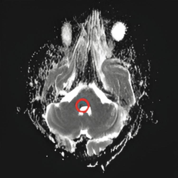
This diagnostic image is an axial Apparent Diffusion Coefficient (ADC) map from a brain Magnetic Resonance Imaging (MRI) study. The image shows the posterior fossa at the level of the brainstem and cerebellum. A red circle highlights a focal area of decreased signal intensity (hypointensity) within the brainstem. This hypointense signal on an ADC map, when correlated with hyperintensity on diffusion-weighted imaging (DWI), confirms true diffusion restriction, which is a hallmark finding of acute ischemic stroke (infarction). The surrounding cerebellar tissue displays intermediate signal intensity, while the fourth ventricle is visible as a high-signal (bright) area posterior to the brainstem. This image is used in clinical neurology and radiology to differentiate acute cerebral infarction from other pathologies by confirming cytotoxic edema.

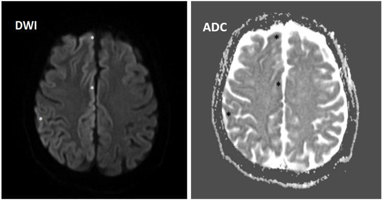
This diagnostic image consists of two axial MRI brain scans side-by-side, displaying Diffusion-Weighted Imaging (DWI) on the left and an Apparent Diffusion Coefficient (ADC) map on the right. The images demonstrate focal areas of true diffusion restriction within the cortical ribbon and sulci of the right frontal and parietal lobes. On the DWI sequence, these areas present as hyperintense (bright) signals, marked with asterisks. Correspondingly, the ADC map shows hypointense (dark) signals in the exact same anatomical locations, confirming restricted diffusion rather than T2 shine-through. This 'cortical ribboning' pattern is a classic radiological finding often associated with rapidly progressive dementias such as Creutzfeldt-Jakob Disease (CJD), or alternatively, acute ischemic stroke or post-ictal states. The visual comparison between the high DWI signal and low ADC signal is essential for identifying cytotoxic edema and abnormal protein deposition in neurodegenerative pathology.

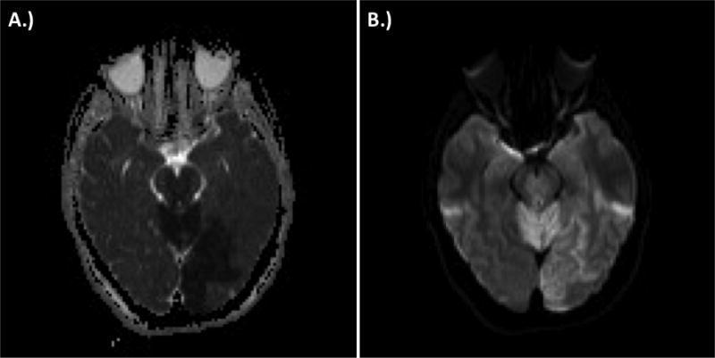
Two axial MRI sequences of the brain demonstrating an acute ischemic stroke within the posterior circulation territory. Figure A shows an Apparent Diffusion Coefficient (ADC) map, while Figure B displays Diffusion-Weighted Imaging (DWI). In the ADC map (A), there are regions of low signal intensity (dark) in the left occipital lobe, signifying restricted water diffusion. Correspondingly, the DWI sequence (B) reveals hyperintense (bright) signals in the same left occipital region, as well as extensive involvement of the cerebellum and brainstem (pons and medulla). This contrast mismatch—hypointensity on ADC and hyperintensity on DWI—is the hallmark of acute cytotoxic edema and infarction. The anatomical distribution follows the posterior circulation, consistent with vascular occlusion affecting the vertebrobasilar system and posterior cerebral arteries. This visual illustrates the diagnostic utility of diffusion restriction in identifying acute cerebral ischemia shortly after an event.

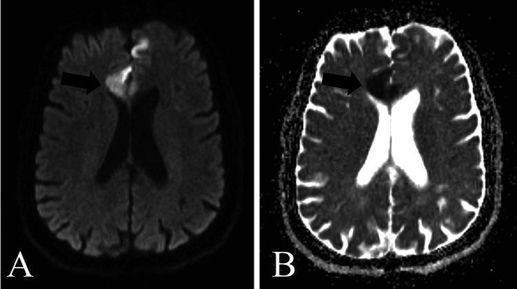
This diagnostic image displays a side-by-side comparison of axial brain MRI sequences, specifically Diffusion-Weighted Imaging (DWI) (A) and the corresponding Apparent Diffusion Coefficient (ADC) map (B). The images demonstrate bilateral frontal lobe pathology, characterized by focal areas of hyperintensity on DWI (A) and corresponding hypointensity on the ADC map (B). This visual pattern represents 'true diffusion restriction,' a finding commonly associated with cytotoxic edema, acute ischemic stroke, or inflammatory processes such as encephalitis. Anatomical landmarks including the lateral ventricles, cerebral hemispheres, and interhemispheric fissure are visible. In the DWI sequence, the ventricles appear hypointense, whereas in the ADC map, the cerebrospinal fluid exhibits high signal intensity. The visual evidence of restricted diffusion in the frontal regions serves as a critical diagnostic indicator for acute neurological conditions requiring immediate clinical correlation.

Finding Sources

Searching Images

DTI tractography white matter fiber tracts brain diffusion tensor imaging

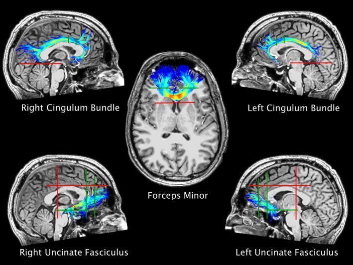
This diagnostic image set showcases Diffusion Tensor Imaging (DTI) tractography of white matter bundles in a template human brain. The figure consists of five panels: four sagittal views and one central axial view, each displaying specific fiber tracts overlaid on a T1-weighted anatomical grayscale background. The sagittal views highlight the bilateral Cingulum Bundles (top) following the curvature above the corpus callosum, and the bilateral Uncinate Fasciculi (bottom) connecting the temporal and frontal lobes. The central axial view depicts the Forceps Minor, extending through the genu of the corpus callosum. The tracts are color-coded with a blue-to-yellow gradient, representing fiber orientation or streamline density. Superimposed red and green straight lines denote 'NOT-regions of interest (ROIs)' and 'AND-ROIs' respectively, which are used as anatomical constraints for the deterministic or probabilistic tractography algorithms. This visualization is essential for neuroanatomical education and clinical research into traumatic brain injury (TBI) and white matter integrity.

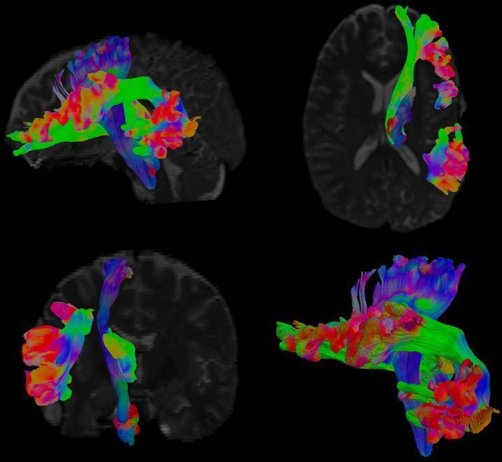
This diagnostic image displays Diffusion Tensor Imaging (DTI) tractography of the human brain across four views: sagittal, axial, coronal, and a 3D oblique reconstruction. The visualization uses a standard RGB color-coding system to represent the orientation of white matter fiber bundles: red for left-right, green for anterior-posterior, and blue for superior-inferior directions. The image specifically highlights major white matter tracts, including the anterior thalamic radiation (depicted in blue/purple tones in the context of connectivity) and the corticospinal tract. The tracts are shown as reconstructed 3D streamlines superimposed on grayscale anatomical MRI backgrounds. This educational content illustrates neuroanatomy and connectivity, specifically focusing on how geometric features of tracts, such as thickness and length, correlate with clinical psychological symptoms like somatization and anxiety. The dense, fiber-like structures demonstrate the complex spatial arrangement of the internal capsule and various radiations connecting the thalamus to the cerebral cortex and brainstem.

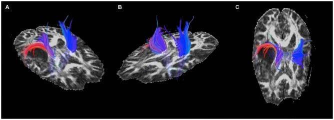
This diagnostic image set presents pre-operative Diffusion Tensor Imaging (DTI) fiber tractography overlaid on axial and oblique T1-weighted anatomical brain MRI slices. The visualization displays white matter pathways, specifically the corona radiata and sensorimotor tracts, categorized into blue and red colored fiber bundles. Panel (A) and (C) demonstrate a pathologic state in the right hemisphere where a visible astrocytoma causes significant mass effect. The red-colored fiber tracts are clearly displaced, exhibiting a curved morphology as they course around the posterior-superior aspect of the tumor. Concurrently, the blue-colored tracts in these panels show signs of distortion and compression adjacent to the lesion. In contrast, Panel (B) serves as a comparison showing the unaffected left hemisphere, where the blue fiber tracts maintain a normal anatomical distribution and vertical orientation without the lateral displacement or color-coded bundle deviation seen in the right hemisphere. This DTI study illustrates the clinical significance of tractography in preoperative planning, specifically for identifying the relationship between critical motor/sensory white matter pathways and infiltrative brain tumors.

Excellent material retrieved. Here is the complete, detailed explanation.

DWI, ADC, DTI, and Diffusion Restriction in MRI

The Underlying Principle: Brownian Motion of Water

All diffusion sequences are based on one physical phenomenon - the random (Brownian) motion of water molecules in tissue.

In biological tissues, water molecules constantly move randomly. The rate and direction of this movement depends on the tissue microstructure:

Free fluid (CSF): Water molecules move fast and freely in all directions - high diffusion
Normal brain tissue: Moderate diffusion, some restriction by cell membranes
Tightly packed cells / cytotoxic edema: Water molecules are trapped inside swollen cells - very little movement - restricted diffusion
White matter axons: Water moves more easily along the axon than across it - anisotropic diffusion

1. DWI - Diffusion-Weighted Imaging

What is it?

DWI is a modified T2-weighted EPI (echo-planar imaging) sequence that adds pairs of strong magnetic field gradients to detect water molecule movement. It is the most clinically used diffusion sequence.

How it works - the physics

The sequence applies:

A standard T2-weighted spin-echo base sequence
Two equal, paired diffusion-sensitizing gradient pulses placed either side of the 180° refocusing pulse

Here is what happens:

Molecules that MOVE: The two gradients don't cancel each other out completely because the protons have moved between pulses → dephasing → signal LOSS → appears DARK
Molecules that DON'T MOVE (restricted): The two gradients cancel perfectly → no dephasing → signal PRESERVED → appears BRIGHT

The key insight: Restricted diffusion = bright on DWI. Free diffusion = dark on DWI.

The b-value

The b-value is the key parameter that controls how strongly the sequence is sensitized to diffusion:

$$b = \gamma^2 G^2 \delta^2 \left(\Delta - \frac{\delta}{3}\right)$$

In simple terms: higher b-value = stronger diffusion weighting

b-value	Meaning	CSF appearance
b=0	No diffusion weighting (standard T2)	Bright
b=500	Mild diffusion weighting	Intermediate
b=1000	Standard DWI in clinical brain imaging	Dark
b=2000+	High b - very sensitive to restriction	Very dark

At b=1000 (standard), CSF is nearly black (high diffusion), normal brain is mid-grey, and acutely ischemic/infected/hypercellular tissue is bright white.

What DWI actually shows

DWI signal = a combination of T2 signal + diffusion information. This creates a potential problem called T2 shine-through.

2. ADC Map - Apparent Diffusion Coefficient

Why ADC is needed - solving T2 shine-through

A lesion with a very long T2 (e.g., a cyst) can appear bright on DWI simply because of T2 effect, NOT because of true restricted diffusion. This is called T2 shine-through - it's a false positive.

The ADC map eliminates this problem.

What is ADC?

The ADC is calculated by acquiring DWI at at least two different b-values (e.g., b=0 and b=1000) and computing the rate of signal decay between them:

$$ADC = -\frac{\ln(S_{b1000} / S_{b0})}{b_{1000} - b_0}$$

The ADC map is a quantitative map showing the actual rate of water diffusion, independent of T2 effects.

High ADC value = fast diffusion = bright on ADC map
Low ADC value = slow/restricted diffusion = dark on ADC map

The DWI/ADC pairing rule - CRITICAL

Finding	DWI	ADC	Interpretation
True restriction	BRIGHT	DARK	True restricted diffusion (stroke, abscess, hypercellular tumor)
T2 shine-through	Bright	Bright or normal	Not true restriction - just T2 effect (cyst, hemangioma)
T2 blackout (T2 dark)	May appear dark	May appear bright	Due to very short T2 (hemosiderin, calcification)

Always interpret DWI together with ADC. Bright DWI + Dark ADC = TRUE restricted diffusion.

Acute ischemic stroke: ADC map showing dark hypointense area in left occipital lobe (restricted), DWI showing bright hyperintense signal in same region

Classic acute posterior circulation infarct. Left: ADC map - dark areas = restricted diffusion. Right: DWI - bright areas = same territory. This DWI bright + ADC dark pattern confirms acute cytotoxic edema (infarction).

Brainstem infarct: ADC map showing focal hypointensity in brainstem - acute restricted diffusion

ADC map - focal dark area in brainstem = acute infarction. High-signal 4th ventricle behind confirms this is truly the ADC map (CSF appears bright on ADC).

3. What is Diffusion Restriction?

Definition

Diffusion restriction means water molecules cannot move freely - they are physically constrained within the tissue. On imaging: bright DWI + dark ADC.

Why does restriction happen - mechanisms

Mechanism	What happens	Example
Cytotoxic edema	Cell death → Na/K pump fails → cells swell → extracellular space shrinks → water trapped intracellularly	Acute stroke
High cell density	Tightly packed cells leave tiny extracellular space - water cannot diffuse	Lymphoma, PNET, medulloblastoma
Viscous protein-rich fluid	Thick macromolecules obstruct free water movement	Abscess pus, epidermoid contents
Intact myelin barriers	Normally confines diffusion, loss of myelin (demyelination) can change diffusion patterns	MS, active demyelination

Clinical causes of diffusion restriction

Condition	DWI	ADC	Notes
Acute ischemic stroke	Bright	Dark	Within minutes of onset; persists ~7-10 days
Cerebral abscess	Bright (central)	Dark	Pus is viscous - classic finding; helps differentiate from necrotic tumor
Epidermoid cyst	Bright	Dark	Keratin debris; distinguishes from arachnoid cyst (no restriction)
CNS lymphoma	Bright	Dark	High cellular density
Glioblastoma (cellular zones)	Bright	Dark	Markedly reduced diffusivity
Diffuse axonal injury (DAI)	Bright	Dark	Shear injury at grey-white junction, corpus callosum
Creutzfeldt-Jakob disease (CJD)	Bright	Dark	Cortical ribboning + basal ganglia restriction
Acute demyelination (MS)	Bright	Dark	Active MS plaques
Hypercellular tumors	Bright	Dark	Medulloblastoma, PNET

Per Bradley and Daroff's Neurology: "Examples include abscesses, hypercellular tumors such as lymphoma, some meningiomas, epidermoid cysts, aggressive demyelinating disease, and proteinaceous material."

Per Grainger & Allison's: "Acute cerebral infarcts show restricted diffusion (high DWI signal, low ADC values) within minutes of onset, as do regions of active demyelination, infections (e.g. cerebral abscess) and cellular tumours (glioblastoma and lymphoma)."

The DWI/FLAIR mismatch rule in stroke

Per Rosen's Emergency Medicine and current stroke guidelines:

DWI bright + FLAIR negative = stroke onset likely <4.5-6 hours (the infarct core is established but vasogenic edema hasn't developed yet - tissue potentially salvageable)
DWI bright + FLAIR bright = stroke onset likely >6 hours (FLAIR has become positive, suggesting older ischemia)

This mismatch is used to select patients with unknown onset or wake-up strokes for thrombolysis or thrombectomy.

DWI and ADC showing bilateral frontal restriction in acute encephalitis - bright DWI, dark ADC bilaterally

Bilateral frontal bright DWI + dark ADC = true restriction. This pattern can represent acute stroke, encephalitis, or other causes of cytotoxic edema.

Cortical ribboning on DWI and ADC - asterisks showing cortical restriction in right frontal/parietal lobes - CJD pattern

Cortical ribboning - DWI bright and ADC dark along the cortical ribbon. This pattern (right frontal/parietal here) is classic for Creutzfeldt-Jakob disease (CJD) or can be seen in post-ictal states.

4. DTI - Diffusion Tensor Imaging

What is DTI?

DTI is an advanced extension of DWI that measures diffusion in at least 6 different directions (typically 12-64 directions), allowing it to characterize not just the magnitude of diffusion but also its directionality.

Per Grainger & Allison's: "Diffusion tensor imaging (DTI) incorporates additional diffusion directions (6+) to gain information about the directionality of water diffusion."

The key concept: Anisotropy

Isotropic diffusion: Water moves equally in all directions (e.g., CSF in a large cistern). Represented as a sphere.

Anisotropic diffusion: Water moves preferentially in one direction more than others. Represented as an ellipsoid.

In white matter axons, diffusion is highly anisotropic:

Water moves freely ALONG the axon (parallel to myelin sheath)
Water is restricted ACROSS the axon (perpendicular, blocked by myelin)

DTI measures the full 3D diffusion tensor - a mathematical ellipsoid describing direction and magnitude of diffusion at each voxel.

Key DTI metrics

Metric	What it measures	Normal value	Clinical meaning
FA (Fractional Anisotropy)	How directional is diffusion? 0=isotropic sphere, 1=fully directional line	WM: 0.3-0.8; GM: ~0.1	Low FA = disrupted white matter (injury, infiltration, demyelination)
MD (Mean Diffusivity)	Average rate of diffusion in all directions	Similar to ADC	High MD = tissue destruction/edema
Axial Diffusivity (AD)	Diffusion along the principal axis (along axon)		Reduced in axonal injury
Radial Diffusivity (RD)	Diffusion perpendicular to the principal axis		Increased in demyelination
ADC (trace)	Mean of all three eigenvalues		Same as DWI ADC

Tractography

Using the directional information from DTI, computer algorithms can trace the path of white matter fiber bundles through the brain. This is called tractography (or fiber tracking).

Deterministic tractography: Follows the principal diffusion direction step by step through voxels
Probabilistic tractography: Accounts for uncertainty and produces a probability map of fiber paths

The result is a colorful 3D map of white matter tracts, color-coded by direction:

Red = left-right fibers (commissural tracts, corpus callosum)
Green = anterior-posterior fibers (association tracts, cingulum, uncinate)
Blue = superior-inferior fibers (corticospinal tract, internal capsule)

DTI tractography showing white matter bundles - cingulum bilaterally and uncinate fasciculi - color-coded by fiber orientation

DTI tractography showing cingulum bundles (top, arching above corpus callosum) and uncinate fasciculi (bottom, connecting frontal and temporal lobes). Color gradient shows fiber orientation and density.

DTI tractography showing corticospinal tract displaced by brain tumor - red fibers deviated around right hemisphere astrocytoma

Pre-operative DTI tractography. Left panels: right hemisphere with astrocytoma - red motor tract fibers are clearly displaced and curved around the tumor. Right panel: normal left hemisphere for comparison. Essential for safe surgical planning.

Clinical uses of DTI

Application	How DTI helps
Pre-operative surgical planning	Map corticospinal tract, arcuate fasciculus, optic radiations relative to tumor - guides safe resection
Brain tumor characterization	Tumor infiltration destroys FA; tract displacement vs. infiltration
Traumatic brain injury (TBI) / DAI	Low FA in white matter tracts indicates axonal damage even when conventional MRI is normal
Multiple sclerosis	FA reduction in normal-appearing white matter (NAWM); progression marker
Stroke	Wallerian degeneration of corticospinal tract - poor FA predicts poor motor recovery
Epilepsy	Map optic radiations before temporal lobectomy (to preserve vision)
Neurodegenerative diseases	ALS (corticospinal FA), frontotemporal dementia (frontal tract FA)
Research / connectomics	Mapping the human connectome - all white matter connections

Per Grainger & Allison's: "Tractography is used widely for preoperative planning, as it helps to depict the relations between intrinsic brain tumours and surrounding neural connections."

Per Kaplan & Sadock's: "Diffusion tensor tractography, which allows visualization and analysis of specific white matter pathways, may extend the potential of DTI in TBI. However, DTI and tractography techniques are primarily reserved for the research setting due to varying methodologies among investigators and lacking normative data."

DTI 4-view tractography showing complete white matter tract system - sagittal, axial, coronal, and 3D oblique views, color-coded red/green/blue by direction

Full DTI tractography in 4 views. Red = left-right (corpus callosum), Green = front-back (association fibers), Blue = up-down (corticospinal tract, internal capsule). This color system is universal in DTI imaging.

5. DWI Beyond the Brain - Body DWI

DWI is not just for the brain. It is increasingly used throughout the body:

Location	Application
Liver	Tumor characterization - cellular tumors restrict (HCC, mets, lymphoma); cysts don't restrict
Prostate	PI-RADS scoring - low ADC in peripheral zone = suspect prostate cancer
Whole body DWI	Bone metastasis detection (replacing bone scan in some centers)
Lymph nodes	Malignant nodes restrict diffusion; ADC may help differentiate reactive vs malignant
Abdomen	Abscess vs cyst, bowel ischemia, renal masses

Per Yamada's Gastroenterology: "Cellular tissues, such as tumors or abscesses, will demonstrate restricted diffusion (high signal intensity) on higher b value (≥500 s/mm²) images and lower ADC values. By contrast, cystic or necrotic tissues will show a greater degree of signal attenuation."

6. Summary: DWI vs DTI vs ADC

Feature	DWI	ADC Map	DTI
What it measures	Restriction of diffusion	Quantitative diffusion rate	Directional diffusion tensor
b-values used	0 + 1000 (typically)	Calculated from ≥2 b-values	6-64 directions + multiple b-values
Key output	DWI image	ADC value (mm²/s)	FA map, tractography
Restricted diffusion appears	Bright	Dark	N/A
CSF appears	Dark (b=1000)	Bright (high ADC)	Isotropic (FA ~0)
Primary clinical use	Acute stroke, abscess, tumor	Confirm true restriction; quantify	Surgical planning, white matter integrity
Limitation	T2 shine-through	-	Motion-sensitive, long acquisition

7. Quick Memory Rules

DWI bright + ADC dark = TRUE RESTRICTION (stroke, abscess, lymphoma, epidermoid)
DWI bright + ADC bright = T2 SHINE-THROUGH (cyst, hemangioma - NOT true restriction)

DWI + FLAIR negative = Stroke within ~4.5-6 hours → Consider thrombolysis
DWI + FLAIR positive = Stroke likely >6 hours → Beyond thrombolysis window

DTI = DWI in 6+ directions → measures DIRECTION of diffusion
FA high = intact white matter | FA low = damaged/infiltrated white matter
Tractography = tracing fiber bundles using DTI directionality data

Explain advanced perfusion imaging techniques (DSC, DCE, ASL)

These are the three core MRI perfusion techniques used in neuro-oncology, stroke, and body imaging. Let me pull the textbook content first.

Searching sources...

Finding Sources

Reading File

Finding Sources

Searching Images

MRI perfusion CBV CBF MTT maps stroke penumbra infarct core

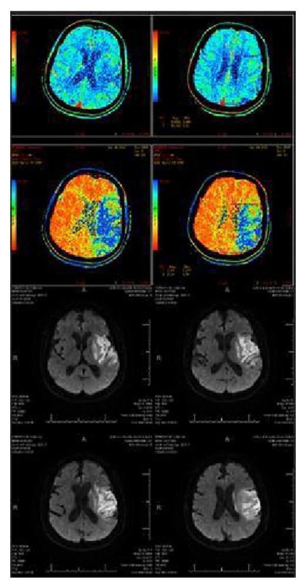
A multi-panel neuroimaging collage illustrating the radiographic assessment of acute ischemic stroke and penumbral mismatch. The top four panels display axial CT Perfusion (CTP) color maps. The uppermost row shows relatively uniform blue hues representing preserved Cerebral Blood Volume (CBV), while the second row exhibits large areas of orange and red signal in the left hemisphere, indicating prolonged Mean Transit Time (MTT) or reduced Cerebral Blood Flow (CBF). This perfusion-diffusion mismatch identifies the 'tissue at risk' or ischemic penumbra. The bottom four panels present axial Diffusion-Weighted Imaging (DWI) MRI sequences taken 24 hours post-intervention. These images show a localized region of hyperintensity (bright signal) in the left frontoparietal and subcortical regions, representing the final infarct core or completed stroke. Comparing the large area of perfusion abnormality on CTP to the smaller restricted diffusion area on MRI allows for the calculation of percentage area salvage, a key metric in evaluating the efficacy of mechanical thrombectomy.

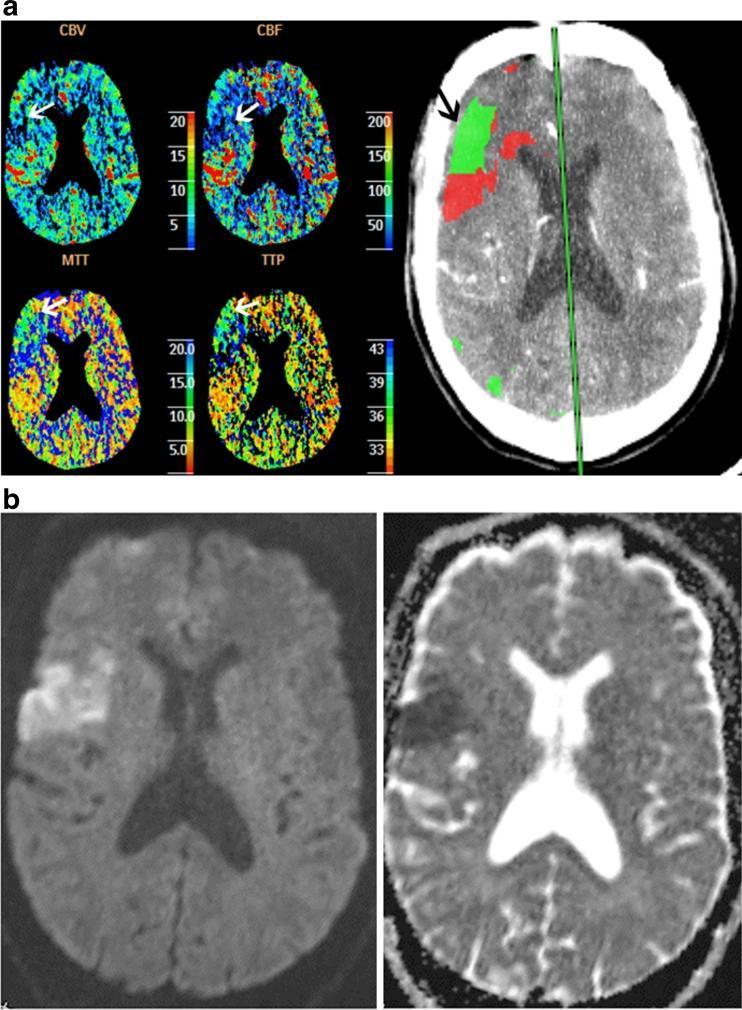
Educational diagnostic imaging series demonstrating acute cerebral infarction evaluation using CT Perfusion (CTP) and MRI. (a) Axial CTP maps (CBV, CBF, MTT, and TTP) show a perfusion deficit in the right middle cerebral artery (MCA) territory, indicated by open arrows. The area of abnormality progressively increases from CBV to TTP, illustrating a perfusion mismatch. A large-scale computer-generated lesion map (closed arrow) identifies a 'mixed lesion' with red indicating the infarct core (decreased CBV) and green representing the ischemic penumbra (elevated MTT with normal CBV). (b) Follow-up MRI performed 4 hours later includes Diffusion-Weighted Imaging (DWI) and an Apparent Diffusion Coefficient (ADC) map. These confirm an acute infarct in the right hemisphere, characterized by high signal on DWI and corresponding low signal on ADC, matching the initial CBV deficit on CTP. The image serves to teach the concepts of infarct core versus penumbra and the correlation between CTP parameters and definitive MRI evidence of ischemia.

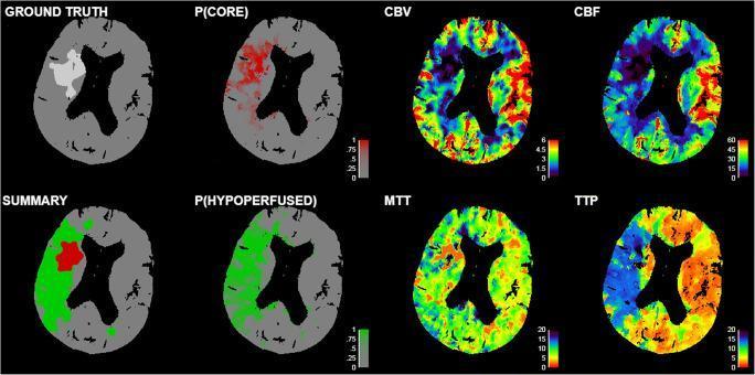
This diagnostic image set displays a series of axial CT perfusion maps and predictive models for an acute ischemic stroke. The panels are organized into ground truth, probability models, and raw perfusion parameters. The 'Ground Truth' and 'Summary' maps highlight the core infarct (red) and the surrounding hypoperfused penumbra (green) in the left hemisphere. Two probability maps, P(CORE) and P(HYPOPERFUSED), use red and green gradients respectively to illustrate the likelihood of tissue infarction based on recanalization status. The four perfusion maps demonstrate classic ischemic signatures: Cerebral Blood Flow (CBF) and Cerebral Blood Volume (CBV) show significant reductions (cool colors/darker blues) in the affected territory, while Mean Transit Time (MTT) and Time to Peak (TTP) show corresponding prolongations (warm colors/yellow-red), indicating delayed contrast arrival and transit. These maps are used in neurology and radiology to assess tissue viability and differentiate salvageable penumbra from the irreversible ischemic core, guiding treatment decisions such as thrombectomy or thrombolysis.

Finding Sources

Searching Images

DCE MRI Ktrans pharmacokinetic model tumor permeability perfusion

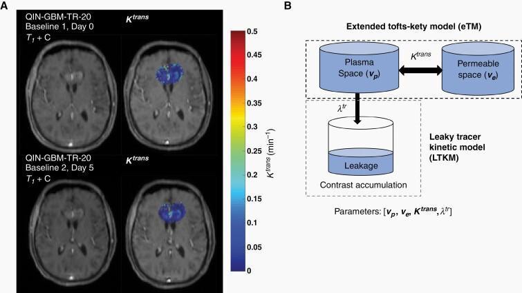
This figure presents clinical diagnostic imaging and a pathophysiology diagram related to neuro-oncology and perfusion MRI. Panel A displays axial T1-weighted post-contrast Dynamic Contrast-Enhanced MRI (DCE-MRI) scans and corresponding parametric maps of the volume transfer constant (Ktrans) for a glioblastoma patient (QIN-GBM-TR-20) at two time points: Baseline 1 (Day 0) and Baseline 2 (Day 5). The parametric maps utilize a color-coded heat map (scale 0 to 0.5 min⁻¹) to illustrate localized areas of high vascular permeability, primarily located in the central periventricular region. Panel B is a compartmental model diagram contrasting the Extended Tofts-Kety Model (eTM) with the Leaky Tracer Kinetic Model (LTKM). It illustrates the exchange between the plasma space (vp) and the extravascular extracellular space (ve) via Ktrans, while the LTKM introduces an additional leakage compartment governed by the rate constant λtr. This educational material focuses on the quantitative assessment of tumor hemodynamics and the repeatability of pharmacokinetic modeling in brain tumor imaging.

$A series of nine axial dynamic contrast-enhanced (DCE) MRI parametric maps illustrating tumor permeability and perfusion in a C6 glioma model. The images are arranged in a grid showing three time points (14 days, 21 days, and 28 days post-transplantation) across columns labeled Vp (plasma volume fraction) and Ktrans (volume transfer coefficient). The color-coded maps utilize a jet scale where blue represents low values and red/yellow represents high values. At 14d, the Ktrans maps show a central area of low permeability (blue) surrounded by a high-permeability peripheral ring (red/yellow). By 21d, the Ktrans maps demonstrate a significant expansion of the high-permeability red zones, coinciding with increased tumor volume. The Vp maps show a heterogeneous increase in vascular plasma volume at 21d, which appears to become more diffuse and slightly less intense by 28d. These diagnostic images track the longitudinal progression of tumor angiogenesis and vascular permeability within the neuro-oncological context.$

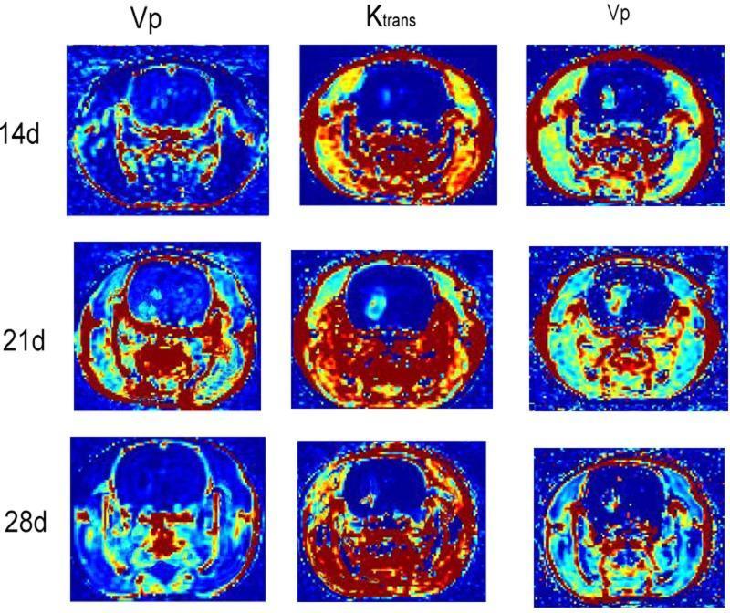
A series of nine axial dynamic contrast-enhanced (DCE) MRI parametric maps illustrating tumor permeability and perfusion in a C6 glioma model. The images are arranged in a grid showing three time points (14 days, 21 days, and 28 days post-transplantation) across columns labeled Vp (plasma volume fraction) and Ktrans (volume transfer coefficient). The color-coded maps utilize a jet scale where blue represents low values and red/yellow represents high values. At 14d, the Ktrans maps show a central area of low permeability (blue) surrounded by a high-permeability peripheral ring (red/yellow). By 21d, the Ktrans maps demonstrate a significant expansion of the high-permeability red zones, coinciding with increased tumor volume. The Vp maps show a heterogeneous increase in vascular plasma volume at 21d, which appears to become more diffuse and slightly less intense by 28d. These diagnostic images track the longitudinal progression of tumor angiogenesis and vascular permeability within the neuro-oncological context.

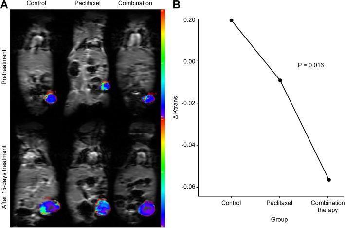
This medical image displays the results of Dynamic Contrast-Enhanced MRI (DCE-MRI) evaluating tumor perfusion in a mouse model. Panel A presents axial Ktrans color-coded maps of three experimental groups—Control, Paclitaxel, and Combination therapy—at two time points: Pretreatment and After 15 days of treatment. In the pretreatment stage, all groups show a similar pattern where tumor margins exhibit higher Ktrans values (indicated by red/green colors), suggesting abundant blood supply, while the central regions show lower values (blue). After 15 days, the Control group shows sustained high peripheral perfusion. In contrast, the Paclitaxel and especially the Combination therapy groups demonstrate a significant reduction in Ktrans values, shifting toward cooler blue tones throughout the tumor mass. Panel B is a line graph showing the mean change in Ktrans (Δ Ktrans) across the three groups (P = 0.016). The graph illustrates a significant downward trend in vascular permeability and perfusion from the Control group to the Paclitaxel group, with the most pronounced decrease occurring in the Combination therapy group, reflecting therapeutic efficacy in inhibiting tumor angiogenesis.

Reading File

Loading Image

Excellent content gathered. Here is the complete, structured explanation.

Advanced MRI Perfusion Imaging: DSC, DCE, and ASL

What is Perfusion Imaging?

Perfusion means blood delivery to tissue at the capillary level. It is different from angiography (which shows large vessels) - perfusion imaging measures microvascular blood flow, volume, and leakage at the tissue level.

The three MRI perfusion techniques differ in what they measure and how they achieve it:

Technique	Contrast used	What it primarily measures	Main mechanism
DSC	Gadolinium (IV)	Blood volume and flow	T2/T2 signal loss*
DCE	Gadolinium (IV)	Vascular permeability	T1 signal gain
ASL	None	Blood flow only	Magnetically labeled water

1. DSC - Dynamic Susceptibility Contrast

Full name

Dynamic Susceptibility Contrast MRI (also called T2*-weighted perfusion MRI or bolus tracking perfusion)

The core principle

When a concentrated bolus of gadolinium passes through brain capillaries, it creates local magnetic field distortions (susceptibility effect) that shorten T2* in surrounding tissue. This causes a transient signal LOSS on T2*-weighted EPI images.

Tissues with more blood flow receive more gadolinium per unit time → greater and faster signal drop.

The key physics: gadolinium in this technique stays intravascular (in normal brain with intact blood-brain barrier). It acts like a susceptibility contrast agent, not a relaxivity agent.

Acquisition technique

A rapid pressure-injected bolus of Gd-based contrast (4-5 mL/sec) is injected
A T2* EPI sequence repeatedly images a slab of brain every ~1-2 seconds
Signal intensity in each voxel is tracked over ~60-90 seconds
This produces a signal-intensity-time curve for every voxel

In well-perfused tissue:

Signal drops sharply as bolus arrives
Then recovers (signal return) as gadolinium washes out

In hypoperfused tissue:

Smaller, delayed, or absent signal drop

The deconvolution step - AIF

To calculate absolute perfusion parameters, the measured tissue concentration-time curve must be mathematically deconvolved with the Arterial Input Function (AIF) - the concentration-time curve measured in a feeding artery (typically the middle cerebral artery or internal carotid).

This corrects for differences in bolus shape and timing between patients.

DSC-derived perfusion maps

Parameter	What it means	How calculated	Abnormal finding in ischemia
CBV (Cerebral Blood Volume)	Volume of blood per unit mass of tissue (mL/100g)	Area under concentration-time curve	↓ in core infarct
CBF (Cerebral Blood Flow)	Volume of blood flowing through tissue per unit time (mL/100g/min)	CBV/MTT	↓↓ in core
MTT (Mean Transit Time)	Average time for blood to traverse capillary bed (sec)	CBV/CBF	↑ in penumbra and core
Tmax	Time from AIF to peak of tissue residue function (sec)	Deconvolution	>6 sec = penumbra (best marker)
TTP (Time to Peak)	Time from injection to peak signal drop	Directly measured	↑ in hypoperfused tissue

How DSC identifies stroke penumbra

The perfusion-diffusion mismatch concept:

DWI abnormality = INFARCT CORE (irreversibly dead tissue)
PWI (DSC) abnormality = TOTAL HYPOPERFUSED ZONE
Mismatch = PWI - DWI = ISCHEMIC PENUMBRA (at-risk but salvageable tissue)

Large mismatch → significant penumbra → patient likely to benefit from thrombectomy/thrombolysis
No mismatch (DWI = PWI) → no penumbra → limited therapeutic benefit

Per Grainger & Allison's: "Tmax greater than 6 seconds is currently considered the most reliable biomarker of the penumbra... Other markers include delay-corrected MTT when appropriately thresholded at 145% relative to the contralateral normal side."

Perfusion maps (CBV, CBF, MTT, TTP) in acute right MCA territory stroke. CBV and CBF reduced in core (cool blue colors), MTT and TTP prolonged in penumbra (warm colors). DWI confirms final infarct core.

CTP/MR perfusion maps: CBV (reduced = core), CBF (reduced), MTT (prolonged = penumbra), TTP (prolonged). DWI 4 hours later confirms completed infarct in right MCA territory matching the CBV deficit.

Left MCA territory infarct: CTP color maps showing large perfusion abnormality (penumbra) vs small DWI infarct core - large mismatch - patient ideal for thrombectomy

Classic perfusion-diffusion mismatch. CTP (top): large left hemisphere perfusion deficit. DWI (bottom, 24h post-thrombectomy): small residual infarct. The mismatch = salvaged penumbra after successful recanalization.

DSC in neuro-oncology - rCBV

In brain tumors, DSC is used to measure relative Cerebral Blood Volume (rCBV):

High-grade glioma (GBM): High rCBV due to neovascularity (tumor angiogenesis)
Low-grade glioma: Low rCBV
rCBV >1.75 relative to normal white matter = suggests high-grade tumor
Pseudoprogression (treatment effect) vs. true tumor progression: rCBV is low in pseudoprogression, high in true recurrence

Per Grainger & Allison's: "DTI-based advanced diffusion methods are being trialled in research to enhance the micro-structural analysis of certain brain tumours" and low ADC values "may help identify malignant gliomas, and markedly reduced diffusivity may define certain neoplasms such as lymphoma."

Clinical uses of DSC

Application	Detail
Acute stroke	Perfusion-diffusion mismatch; identify penumbra for treatment selection
Brain tumor grading	rCBV correlates with tumor grade and angiogenesis
Tumor recurrence vs. treatment effect	High rCBV = recurrence; low rCBV = radiation necrosis/pseudoprogression
Cerebrovascular reserve	After carotid occlusion, Moyamoya
Dementia	Regional hypoperfusion patterns in Alzheimer's, FTD

Limitations of DSC

Requires gadolinium (contrast risks)
Susceptibility artifacts at skull base, near hemorrhage, post-surgical sites (metal/blood products distort the signal)
Assumes intact BBB - leakage correction needed in tumors
AIF selection is technically challenging
Does not work well in tumors without leakage correction - Gd leaks out of tumor capillaries (BBB breakdown) and causes T1 effects that counteract T2* signal loss, artificially reducing the rCBV → must apply pre-loading dose or mathematical correction

2. DCE - Dynamic Contrast Enhanced MRI

Full name

Dynamic Contrast-Enhanced MRI (T1-weighted perfusion)

The core principle - opposite to DSC

DCE uses the T1-shortening effect of gadolinium (not susceptibility). In DCE, gadolinium leaks out of capillaries into the extravascular extracellular space (EES) through the blood-brain barrier (or tumor neovasculature).

Normal brain BBB: Gd stays intravascular → minimal T1 enhancement
Tumor / inflammation: BBB is disrupted → Gd leaks into tissue → T1 signal INCREASES over time

The rate and amount of leakage reveals microvascular permeability.

Acquisition technique

Pre-contrast T1 baseline image acquired
Gadolinium injected at moderate rate (2-3 mL/sec)
Rapid T1-weighted spoiled gradient echo sequence images the tissue every 5-10 seconds for 5-10 minutes
Signal intensity increases over time as Gd accumulates in tissue
A pharmacokinetic model (Tofts model or extended Tofts model) is fitted to the signal-time curve to extract quantitative parameters

DCE pharmacokinetic model (Tofts model)

The model divides tissue into two compartments:

Plasma (Cp)  ←──Ktrans──→  Extravascular Extracellular Space (EES/ve)
     ↑                              ↓
  Blood flow                    Kep = Ktrans/ve

DCE Parameter	Symbol	What it measures	Clinical meaning
Volume transfer constant	Ktrans (min⁻¹)	Rate of Gd transfer from plasma to EES - reflects capillary permeability × surface area	↑ in high-grade tumor, inflammation
Extravascular extracellular volume	ve	Fraction of tissue volume that is EES	Related to tumor cellularity
Rate constant (washout)	Kep = Ktrans/ve	Rate of Gd transfer back from EES to plasma	Washout kinetics
Plasma volume fraction	vp	Fractional volume of blood plasma in tissue	Vascularization
Initial area under curve	IAUC	Gadolinium uptake in first 60s	Empirical perfusion/permeability

$$K^{trans} = \text{rate of leakage across capillary wall}$$

Per Grainger & Allison's: "DCE MR perfusion examines T1 shortening during passage of a pressure-injected Gd-based contrast agent, and this technique can be used to calculate Ktrans, a measure of capillary permeability, increased in the setting of gliomas (that produce vascular endothelial growth factor), metastases and inflammatory lesions."

DCE-MRI Ktrans parametric maps of glioblastoma patient at baseline - color-coded heat map showing high vascular permeability in periventricular tumor region

DCE-MRI Ktrans maps of a GBM patient. Color scale 0-0.5 min⁻¹. Red/yellow = high permeability (active tumor with disrupted BBB). Blue = low permeability. Right: the Extended Tofts-Kety pharmacokinetic model showing plasma (vp) and extracellular extravascular space (ve) compartments.

DCE Ktrans maps of C6 glioma at 14, 21, and 28 days - progressive increase in high-permeability zones as tumor grows, tracking angiogenesis

Serial DCE Ktrans maps tracking tumor angiogenesis over time. Blue = low permeability, Red/Yellow = high permeability. As tumor grows (14d→28d), zones of high Ktrans expand - reflecting progressive BBB disruption by VEGF-driven neovascularization.

Clinical uses of DCE

Application	Detail
Brain tumor grading	Ktrans ↑ in high-grade glioma (VEGF causes leaky vessels)
Treatment response monitoring	Anti-angiogenic therapy (bevacizumab) → ↓ Ktrans = response
Distinguish radiation necrosis vs recurrence	Recurrence: ↑ Ktrans; radiation necrosis: ↓ Ktrans
Prostate cancer	DCE is part of the PI-RADS scoring system (early enhancement = malignancy)
Breast MRI	Kinetic curve shape - rapid uptake + washout = malignant
Cervical/endometrial cancer	Treatment response, lymph node assessment
Multiple sclerosis	Active lesions show Ktrans ↑ (BBB disruption)

DSC vs DCE comparison

Feature	DSC	DCE
MRI weighting	T2* (gradient echo EPI)	T1 (spoiled GRE)
Gadolinium effect	Susceptibility → signal LOSS	T1 shortening → signal GAIN
BBB assumption	Intact BBB (blood stays in vessels)	BBB disruption measured
Primary output	CBV, CBF, MTT	Ktrans, ve, vp
Best for	Stroke, rCBV in tumors	Tumor permeability, treatment response
Time resolution	~1-2 sec (fast)	5-10 sec (moderate)
Scan duration	~2 min	5-10 min

3. ASL - Arterial Spin Labeling

Full name

Arterial Spin Labeling MRI (also called spin-labeled perfusion MRI)

The revolutionary concept - NO contrast needed

ASL is the only perfusion MRI technique that requires no injection of contrast. It uses magnetically labeled water molecules in blood as an endogenous tracer.

How it works - step by step

An inversion pulse (radiofrequency pulse) is applied to a slab of tissue below (proximal to) the imaging slice - typically in the neck (labeling plane)
This inverts the magnetization of water protons in inflowing arterial blood → magnetically tagged blood
A short delay (post-labeling delay, PLD ~1.5-2 sec) allows the labeled blood to travel up into the brain tissue
The imaging slice is acquired → the labeled image
The same process is repeated without the inversion pulse → the control image

$$\text{Perfusion signal} = \text{Control image} - \text{Labeled image}$$

Where labeled blood has arrived, the tissue signal is slightly reduced (inverted protons partially cancel the tissue signal). Subtracting gives a pure perfusion map.

Per Kaplan & Sadock's: "ASL relies on the magnetic labelling/tagging of inflowing blood (such as with an inversion pulse)... Upon subtraction of the pair of images from one another, pixels that represent static brain water will approach zero, but pixels that lie in the path of blood flow will appear up to twice as bright as those in the baseline image."

ASL variants

Type	How labeling is done	Best for
CASL (Continuous ASL)	Continuous long RF pulse applied to neck	High SNR; older technique
PASL (Pulsed ASL)	Short, thick slab inversion pulse	Simpler; less SAR
pCASL (Pseudo-Continuous ASL)	Series of short pulses mimicking continuous	Current gold standard - best SNR + efficiency

ASL output

ASL directly gives a quantitative CBF map (mL/100g/min), which is the same as the CBF derived from DSC but without contrast.

Normal brain CBF: ~50-60 mL/100g/min (grey matter)

The SNR challenge

The perfusion signal in ASL is only 0.5-1.5% of the total tissue signal - extremely small. This requires:

Multiple averages (signal averaging) to boost SNR
EPI readout for fast acquisition
High field strength (3T preferred over 1.5T)

Clinical uses of ASL

Application	Detail
Pediatric patients	No contrast needed - ideal for children
Renal failure	Cannot give gadolinium (nephrogenic systemic fibrosis risk) - ASL is safe
Repeated/serial measurements	Can be done many times without contrast load
Dementia	Regional CBF maps - hypoperfusion patterns (Alzheimer's = parietal/posterior; FTD = frontal)
Epilepsy	Ictal hyperperfusion, interictal hypoperfusion
Stroke	Subacute/chronic stroke; whole-brain perfusion assessment
Tumor	Relative CBF maps without DSC's susceptibility problems
Psychiatric research	Non-invasive longitudinal CBF studies

ASL limitations

Low SNR - signal is very small; noisy in practice
Sensitive to motion (long acquisition with multiple averages)
Transit time effects - labeled blood may not reach distal territory before T1 relaxation (labeled spins decay with T1 ~1.6 sec at 3T) → underestimates CBF in patients with slow flow (elderly, stroke)
Limited slice coverage (though improving with 3D sequences)
Cannot measure BBB permeability (unlike DCE) or blood volume independently

4. Complete Comparison Table

Feature	DSC	DCE	ASL
Contrast agent	Gadolinium (essential)	Gadolinium (essential)	None
MRI sequence	T2* GRE EPI	T1 spoiled GRE	EPI (subtraction)
Mechanism	Susceptibility (signal loss)	T1 shortening (signal gain)	Magnetic labeling of blood
BBB requirement	Intact (or corrected for leakage)	Disrupted BBB measured	N/A
Primary output	CBV, CBF, MTT, Tmax	Ktrans, ve, vp, IAUC	CBF (quantitative)
Time resolution	~1-2 sec	~5-10 sec	3-5 min (averaged)
SNR	High	High	Low (needs averaging)
Contraindications	Renal failure, contrast allergy	Renal failure, contrast allergy	None
Best brain application	Stroke penumbra, tumor rCBV	Tumor permeability, BBB	Dementia, pediatric, no-contrast
Body application	Limited	Prostate, breast, cervix	Limited
Quantitative?	Semi-quantitative (rCBV)	Yes (Ktrans in min⁻¹)	Yes (absolute CBF)

5. Clinical Scenario Decision Guide

Clinical Question	Best Perfusion Technique
Acute stroke: Is there salvageable tissue?	DSC (PWI) + DWI mismatch
Brain tumor: What grade is it?	DSC (rCBV)
Tumor: recurrence or radiation necrosis?	DSC (rCBV) + DCE (Ktrans)
Anti-angiogenic treatment response?	DCE (Ktrans change over time)
Child with brain pathology (no contrast)	ASL
Dementia: regional blood flow pattern?	ASL
Renal failure patient needing perfusion?	ASL
BBB disruption assessment	DCE
Prostate cancer detection (MRI)	DCE (part of mpMRI)
Stroke: chronic hypoperfusion / Moyamoya?	ASL or DSC

6. Summary - How to Remember Them

DSC = Dynamic Susceptibility Contrast
   → Gd bolus → T2* signal LOSS → fast, measures CBV/CBF/MTT
   → Brain: Stroke penumbra, tumor rCBV

DCE = Dynamic Contrast Enhanced
   → Gd slowly leaks → T1 signal GAIN → measures Ktrans (permeability)
   → Brain tumors, prostate, breast - where BBB/vessel leakage matters

ASL = Arterial Spin Labeling
   → NO contrast → magnetically label blood water → subtract label/control
   → Gives CBF only, but completely safe, no contrast needed

Explain Tmax, rCBV, TTP & MRS in MRI in detail

These are advanced quantitative MRI parameters. Let me pull detailed textbook content on all four simultaneously.

Searching sources...

Finding Sources

Reading File

Searching Images

MR spectroscopy NAA choline creatine brain tumor spectrum peaks

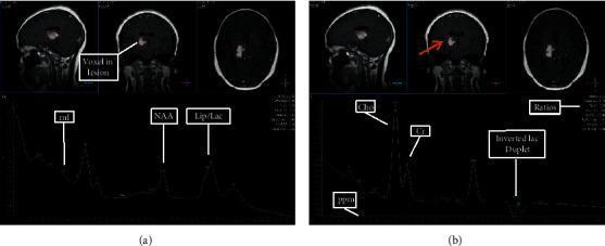
Educational composite featuring brain MRI and Proton Magnetic Resonance Spectroscopy (1H-MRS) used to evaluate high-grade glioma. The top panels show sagittal, coronal, and axial MR views with a single voxel localized precisely within a hyperintense intracranial lesion. The bottom panels present two spectral plots at different echo times (TE): (a) Short TE (31 msec) and (b) Intermediate TE (144 msec). The short TE spectrum highlights peaks for myo-inositol (mI), N-acetylaspartate (NAA), and a combined lipid/lactate (Lip/Lac) peak. The intermediate TE spectrum demonstrates characteristically elevated Choline (Cho) relative to Creatine (Cr) and an inverted lactate doublet at 1.3 ppm, confirming the presence of lactate. Key metabolic findings indicative of high-grade malignancy include a marked elevation in Cho (Cho:Cr ratio 2.93), significant reduction in NAA and myo-inositol, and elevated lipid and lactate levels. This comparison illustrates the diagnostic utility of varying echo times to resolve specific metabolites and assess tumor grade.

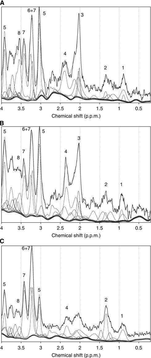
This diagnostic image displays three 1H MR spectra (A, B, and C) comparing metabolic profiles in mouse cerebella across wild-type (WT) and Smoothened (SMO) medulloblastoma models. The x-axis represents the chemical shift in parts per million (p.p.m.), and the y-axis shows signal intensity. Spectrum A (WT) serves as the control, showing prominent peaks for N-acetyl aspartate (NAA at 2.0 p.p.m., label 3), creatine (3.0 p.p.m., label 5), and choline-containing metabolites (3.2 p.p.m., label 6). Spectrum B shows a pre-symptomatic SMO cerebellum with a profile largely similar to the control. Spectrum C illustrates the metabolic hallmark of a T2-hyperintense tumor, characterized by a severe reduction in the NAA peak (marker of neuronal integrity) and a significant elevation in choline (label 6+7) and taurine (label 7) peaks, indicating high cell turnover and tumor progression. Other assigned peaks include lipids/macromolecules (0.9–1.3 p.p.m.), glutamate/glutamine (2.1–2.4 p.p.m.), and glycine/myo-inositol (3.5–3.6 p.p.m.). The visualization demonstrates the utility of magnetic resonance spectroscopy in identifying biochemical biomarkers for pediatric-type brain tumors.

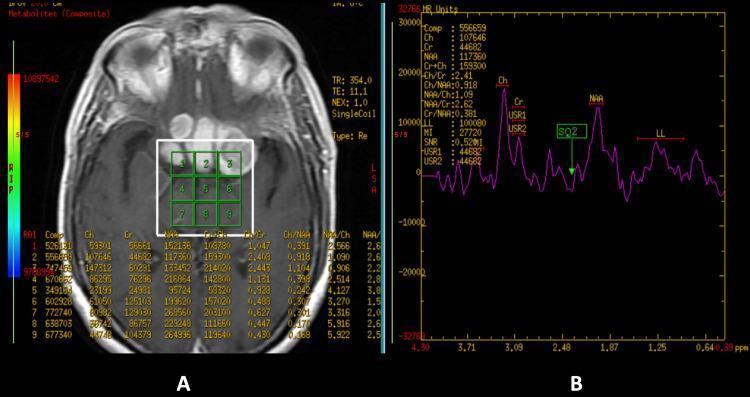
Educational medical graphic presenting Magnetic Resonance Spectroscopy (MRS) of the brain. Panel A shows an axial contrast-enhanced T1-weighted MRI of the brain, highlighting a multi-voxel grid (3x3 region of interest) placed over an intracranial extension in the anterior cranial fossa and suprasellar region. Panel B displays the corresponding MR spectrum, illustrating metabolite peaks at specific parts per million (ppm). The spectrum demonstrates a high Choline (Ch) peak, a stable Creatine (Cr) peak, and a significantly reduced N-acetylaspartate (NAA) peak. These findings result in an elevated Choline-Creatine (Ch/Cr) ratio and a decreased NAA/Cr ratio, characteristic of neoplastic or proliferative processes such as high-grade tumors or specific inflammatory lesions. A Lipid/Lactate (LL) peak is also visible at approximately 1.3 ppm. The display includes quantitative metabolite values and ratios for clinical correlation.

Searching Images

Tmax TTP rCBV perfusion map stroke penumbra color coded brain

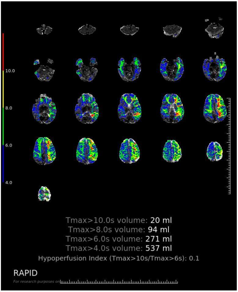
This diagnostic image displays a CT Perfusion (CTP) Tmax map of the human brain, commonly used in the acute management of ischemic stroke to assess the penumbra. The layout consists of multiple axial slices arranged in a grid, showing a large area of hypoperfusion throughout the left cerebral hemisphere. A color-coded scale on the left correlates Tmax values (measured in seconds) with specific colors: blue/green for lower delays (>4s) and yellow/red for higher delays (>10s). The visualization demonstrates an extensive perfusion deficit involving the left middle cerebral artery (MCA) territory. Quantitative data provided at the bottom indicates a tiered volumetric analysis: Tmax >4.0s (537 ml), Tmax >6.0s (271 ml), Tmax >8.0s (94 ml), and Tmax >10.0s (20 ml). A 'Hypoperfusion Index' (Tmax >10s / Tmax >6s) of 0.1 is calculated, which is a clinical metric used to assess the severity of collateral flow failure and predict the rate of infarct core expansion. The educational focus is on identifying tissue at risk versus severely hypoperfused regions using automated RAPID software processing.

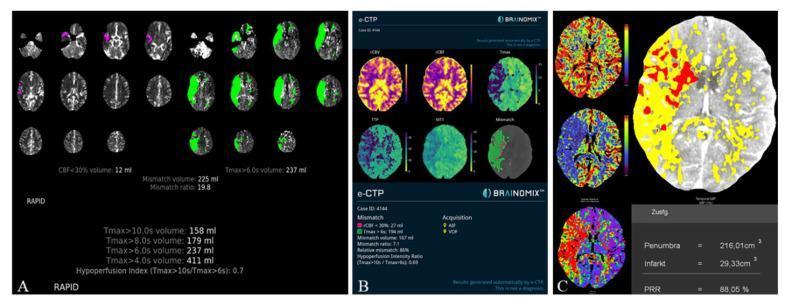
This diagnostic comparison image illustrates automated perfusion CT results for a patient with a right-hemisphere M1-occlusion, processed by three different software packages: RAPID (A), Brainomix (B), and Syngo (C). The composite highlights variations in visual representation and quantitative metrics for acute ischemic stroke. Panel A (RAPID) displays axial brain slices with color-coded maps showing delayed Tmax (>6.0s in green) and severely reduced CBF (<30% in purple), alongside metrics like mismatch volume (225 ml) and Hypoperfusion Index (0.7). Panel B (Brainomix) presents multi-parametric maps (rCBV, rCBF, Tmax, TTP, MTT) with a 167 ml mismatch volume and a Hypoperfusion Intensity Ratio (HIR) of 0.89. Panel C (Syngo) utilizes a large axial slice with a red/yellow overlay to demarcate the infarct core (29.33 cm³) and penumbra (216.01 cm³), showing a Penumbral Salvage Ratio (PRR) of 88.05%. The image demonstrates the clinical utility of automated software in assessing cerebral hemodynamics, identifying salvageable tissue (penumbra), and supporting triage decisions in neuro-radiology.

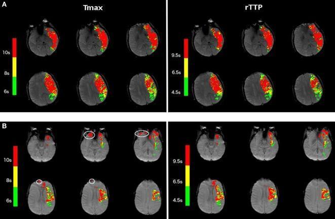
This diagnostic image displays a comparison of Tmax (Time to Maximum) and relative Time to Peak (rTTP) perfusion maps in two acute stroke patients. The image is divided into two sections, A and B, each showing six axial brain slices with color-coded perfusion deficits. In patient example A, there is a clear spatial correspondence between Tmax and rTTP maps, demonstrating high correlation in lesion volume and shape within the left hemisphere. The color scale uses red (severe delay, >10s for Tmax; >9.5s for rTTP), yellow (moderate delay), and green (mild delay, >6s for Tmax; >4.5s for rTTP) to represent hypoperfusion intensity. Example B highlights the susceptibility of different modalities to artifacts; white contours on the Tmax map identify small, localized artifacts that are absent or less prominent on the corresponding rTTP map. These maps are critical in neuroradiology for assessing tissue at risk (penumbra) during acute ischemic stroke and evaluating the technical accuracy of perfusion-weighted imaging parameters.

Loading Image

Finding Sources

Excellent content from textbooks and images. Here is the complete, detailed explanation.

Tmax, rCBV, TTP & MRS in MRI - Detailed Guide

Part 1: Tmax (Time to Maximum of the Residue Function)

What is Tmax?

Tmax is a perfusion-weighted MRI parameter derived from DSC (Dynamic Susceptibility Contrast) perfusion imaging. It represents the time delay between the arrival of contrast at the feeding artery (AIF) and when it reaches its peak effect in the tissue.

Formally: Tmax is the time to the maximum of the residue function - derived from mathematical deconvolution of the tissue concentration-time curve with the Arterial Input Function (AIF).

How it is calculated

In DSC perfusion, a gadolinium bolus is injected. The signal intensity drop over time is measured in:

A feeding artery → this gives the AIF (Arterial Input Function) - the bolus shape entering the brain
Each tissue voxel → this gives the tissue concentration-time curve

The tissue curve is then deconvolved with the AIF using mathematical modeling. The resulting function (residue function) tells you:

How efficiently the bolus arrived at the tissue
When it peaked = Tmax

$$\text{Tmax} = \text{Time at which residue function } R(t) \text{ is maximum after deconvolution}$$

What Tmax measures physically

Tmax reflects bolus arrival delay - how long it takes blood (carrying contrast) to travel from the artery to that tissue voxel. It is:

Primarily a measure of transit delay, not just blood flow
More sensitive to upstream vascular obstruction / collateral-dependent supply than CBF or MTT alone
Tmax = 0 in a normal voxel directly perfused; increases as collateral supply lengthens the path

The clinical threshold: Tmax > 6 seconds

Per Grainger & Allison's Diagnostic Radiology: "A Tmax (time to maximum of the residue function) delay of greater than 6 seconds is felt to be a better predictor of critically hypoperfused penumbral tissue that is destined to infarction in the absence of timely reperfusion."

Tmax value	Tissue status
<4 sec	Normal perfusion
4-6 sec	Mild hypoperfusion / benign oligaemia (may not infarct)
>6 sec	Ischemic penumbra (at-risk tissue, likely to infarct without reperfusion)
>8-10 sec	Severely hypoperfused (higher risk of infarction)

Tmax in RAPID software (the clinical tool)

The automated RAPID software (widely used in thrombectomy trials) generates Tmax maps and reports:

Tmax >6s volume = penumbra estimate
DWI core volume = infarct core
Mismatch ratio (Tmax >6s / DWI) ≥1.2 and mismatch volume ≥15 mL = favorable profile for thrombectomy

Tmax perfusion map - large left MCA territory hypoperfusion. Color scale blue/green = mild delay (>4s), yellow/red = severe delay (>10s). Tiered volumes: Tmax>4s: 537mL, Tmax>6s: 271mL, Tmax>8s: 94mL, Tmax>10s: 20mL

RAPID-processed Tmax map. Large left MCA territory: 271 mL at Tmax>6s (penumbra). The Hypoperfusion Index (Tmax>10s / Tmax>6s) = 0.1, suggesting good collateral flow. Color scale: green = >6s, yellow = >8s, red = >10s delay.

Comparison of RAPID, Brainomix, Syngo software outputs for rCBV, rCBF, Tmax, TTP, MTT maps in right M1 occlusion stroke

Three different automated perfusion software outputs for the same right M1 occlusion. All show Tmax, TTP, MTT, rCBV, rCBF maps. RAPID (A) shows Tmax>6s = green zone (penumbra) and CBF<30% = purple (core). Demonstrates how same data generates slightly different estimates depending on algorithm.

Tmax vs TTP - key differences

Feature	Tmax	TTP
Requires AIF deconvolution	Yes	No
What it measures	Delay of residue function peak	Time from injection to peak signal drop
Sensitivity to bolus dispersion	Lower (corrected by deconvolution)	Higher (influenced by dispersion + transit time)
Variability	More sensitive to AIF selection errors	Less variable across platforms
Clinical threshold	>6 sec = penumbra	3-5 sec delay used in some centers
Use in trials	Used by DEFUSE-3, DAWN trials (RAPID)	Used in older literature

Part 2: TTP (Time to Peak)

What is TTP?

TTP is the simpler, deconvolution-free perfusion parameter. It measures the time from contrast injection (or start of imaging) to the moment the DSC signal reaches its minimum (i.e., the peak of contrast concentration in that voxel).

Per Grainger & Allison's: "Time to peak (TTP) is a perfusion parameter that theoretically could be superior to Tmax for assessment of critically hypoperfused tissue because it does not require deconvolution and, therefore, is not dependent on an AIF."

How it is measured

From the raw DSC signal-intensity-time curve for each voxel:

Signal starts at baseline (bright on T2*)
Signal drops as gadolinium bolus arrives (susceptibility effect)
Signal reaches its minimum → this time point = TTP

$$\text{TTP} = \text{time from start of imaging to minimum signal intensity in the voxel}$$

What TTP reflects

TTP reflects a sum of three effects:

Bolus arrival delay (same as Tmax - upstream vascular delay)
Arterial dispersion (broadening of the bolus as it travels)
Tissue transit time (time for blood to pass through capillaries)

This makes TTP less specific than Tmax but also more robust (less sensitive to AIF errors).

Clinical interpretation

TTP finding	Interpretation
TTP prolonged by 3-5 sec vs. contralateral side	Suggests penumbral hypoperfusion (CBF <20 mL/100g/min)
TTP prolonged >5-6 sec	Higher risk of infarction
Normal TTP bilaterally	No significant perfusion delay

TTP vs Tmax - practical point

In stroke imaging, Tmax is preferred in modern practice (more specific, used in trial protocols)
TTP is still clinically useful where AIF-based deconvolution is not available or is technically limited (e.g., very slow flow, proximal occlusions distorting AIF)
Some older perfusion software reports TTP rather than Tmax

Tmax vs rTTP comparison maps in two acute stroke patients showing close spatial correspondence of penumbral zones, with Tmax more susceptible to artifactual distortions

Side-by-side Tmax (left) and rTTP (right) maps in two stroke patients. In Patient A: excellent spatial correspondence. In Patient B: Tmax shows small white-contoured artifacts (AIF sensitivity) absent on rTTP - demonstrating TTP's robustness. Color: green = mild delay, yellow = moderate, red = severe.

Part 3: rCBV (relative Cerebral Blood Volume)

What is rCBV?

rCBV = relative Cerebral Blood Volume

It is the volume of blood present per unit mass of brain tissue, expressed relative to a reference region (usually contralateral normal white matter), measured from DSC perfusion MRI.

$$rCBV = \frac{CBV_{tissue}}{CBV_{reference\ white\ matter}}$$

Units: dimensionless ratio (or the absolute CBV is in mL/100g)

The "r" (relative) is used because absolute CBV quantification requires a precise AIF calibration, which is difficult in practice. rCBV is easier to calculate and clinically more reproducible.

How rCBV is calculated from DSC

CBV is calculated as the area under the gadolinium concentration-time curve in each voxel:

$$CBV \propto \int_0^\infty C_{tissue}(t), dt$$

In well-perfused tissue, more blood passes through → larger area under the curve → higher CBV.

Normal values

Normal grey matter CBV: ~4-6 mL/100g
Normal white matter CBV: ~2 mL/100g
rCBV (grey/white) ≈ 2 (reference)
Tumor threshold: rCBV >1.75 (relative to normal WM) = suggests high-grade

rCBV in brain tumors - the key clinical use

Tumor angiogenesis creates abnormal, leaky new vessels (driven by VEGF). This increases the density and volume of blood vessels in and around the tumor → elevated rCBV.

Tumor type	rCBV	Why
GBM (Grade 4)	Very high (>4-6×)	Intense angiogenesis, leaky neovascularity
Anaplastic glioma (Grade 3)	High (2-4×)	Active but less intense neovascularization
Low-grade glioma (Grade 2)	Low-normal (1-2×)	Minimal neovascularization
Lymphoma	Variable (moderate)	Hypercellular; may have disrupted BBB
Metastasis	High in solid part	Leaky vessels from primary tumor
Radiation necrosis	LOW	Damaged vessels, no active angiogenesis
Pseudoprogression	Low-intermediate	Treatment effect, not true growth
Meningioma	Very high	Highly vascular tumor

rCBV: Key clinical decision: Recurrence vs. Radiation necrosis

One of the most important uses of rCBV:

Finding	rCBV	Interpretation
Post-treatment enhancing lesion + HIGH rCBV	High (>2.6)	True tumor recurrence/progression
Post-treatment enhancing lesion + LOW rCBV	Low (<1.5)	Radiation necrosis / pseudoprogression

Note: In DSC for tumors, leakage correction is required because the BBB is broken down in high-grade tumors. Without correction, gadolinium leaks into the EES and causes T1 shortening that counteracts the T2* susceptibility effect, underestimating rCBV. Pre-bolus injection (pre-leakage saturation) or mathematical leakage correction algorithms are used.

rCBV in stroke

In acute stroke:

Infarcted core: rCBV low (irreversible ischemia, capillary collapse)
Penumbra: rCBV may be normal or mildly reduced (autoregulation maintains volume despite reduced flow)
Benign oligaemia: rCBV normal or slightly increased (compensatory vasodilation)

The fact that CBV remains relatively preserved in the penumbra (unlike CBF and MTT) is why CBV threshold (not CBV alone) defines the core in CTP.

Part 4: MRS - Magnetic Resonance Spectroscopy

What is MRS?

MRS is a non-invasive technique that measures the chemical composition of tissue by detecting NMR signals from metabolites. Instead of producing a spatial image, it generates a spectrum - a graph of signal amplitude vs. chemical shift (frequency in ppm).

Per Grainger & Allison's: "MRS is a technique that allows non-invasive detection and quantification of tissue metabolites. The identification of the metabolite peaks is derived from the nuclear resonance frequency exerted by the atomic structure of its constituent molecule."

The physics principle

Every molecule has hydrogen nuclei (protons) in slightly different chemical environments. The local electron cloud around each proton shields it from the external magnetic field to a different degree → protons in different molecules precess at slightly different Larmor frequencies.

This frequency difference (measured in parts per million, ppm relative to a reference standard) creates distinct spectral peaks for each metabolite.

$$\text{Chemical shift (ppm)} = \frac{f_{metabolite} - f_{reference}}{f_{reference}} \times 10^6$$

Types of MRS

Type	Nucleus	What it detects
¹H-MRS (Proton MRS)	Hydrogen	NAA, Cho, Cr, Lac, mI, Glx, lipids - most common clinical use
³¹P-MRS	Phosphorus-31	ATP, phosphocreatine (PCr), phosphomonoesters - energy metabolism
¹⁹F-MRS	Fluorine-19	Pharmacokinetics of fluorinated drugs (5-FU)
¹³C-MRS	Carbon-13	Citric acid cycle, hyperpolarized pyruvate imaging

SVS vs MRSI acquisition

Method	Full name	What it does
SVS	Single Voxel Spectroscopy	One voxel (1-8 cm³) - simple, high quality spectrum
MRSI / CSI	MR Spectroscopic Imaging / Chemical Shift Imaging	Grid of many voxels simultaneously - maps metabolite distribution

The Key Brain Metabolites

1. NAA - N-Acetylaspartate (2.0 ppm)

Largest peak in normal brain spectrum
Found almost exclusively in neurons (neuronal marker)
Reflects neuronal integrity and viability

NAA change	Meaning
↓ NAA	Neuronal loss, death, or dysfunction
↓↓↓ NAA	Major neuronal destruction (infarct, high-grade tumor)
Normal NAA	Neurons intact

Per Harrison's: "NAA is an amino acid derivative that is abundant in neurons... an increase in the ratio of choline to NAA (and even loss of NAA signal entirely) correlates with cancer; tumors biologically are associated with increased cellularity from proliferation and the concurrent exclusion of normal neurons."

2. Cho - Choline (3.2 ppm)

Reflects cell membrane turnover and synthesis
Found in choline-containing molecules (phosphocholine, glycerophosphocholine)
Elevated whenever there is increased cell membrane synthesis or breakdown

Cho change	Meaning
↑ Cho	Active cell proliferation, tumor, demyelination
↑↑ Cho	High-grade tumor (active membrane synthesis)
↓ Cho	Tissue necrosis, abscess, hepatic encephalopathy

3. Cr - Creatine + Phosphocreatine (3.0 ppm)

Reflects cellular energy metabolism
Relatively stable across many conditions → used as an internal reference
All ratios (Cho/Cr, NAA/Cr) use Cr as the denominator

Cr change	Meaning
Relatively stable	Used as reference standard
↓ Cr	Necrosis, hepatic encephalopathy, inborn errors

4. Lactate (1.33 ppm) - doublet, inverted at TE=135-144ms

Product of anaerobic glycolysis
Absent in normal brain (aerobic metabolism dominant)
Appears as an inverted doublet on intermediate TE spectra (TE=135ms)

Lactate finding	Meaning
↑ Lactate in tumor	Anaerobic metabolism, high-grade, necrotic areas
↑ Lactate in stroke	Ischemia → anaerobic glycolysis in penumbra/core
Lactate + lipid	Necrosis, GBM, brain abscess

5. Lipids / Mobile lipids (0.9-1.3 ppm)

Normally absent (lipids are membrane-bound and invisible to MRS)
Free mobile lipids appear when cell membranes break down
Seen in necrosis, high-grade tumor, brain abscess

6. mI - Myo-inositol (3.56 ppm) - only at short TE

Astrocyte marker (predominantly in glial cells)
↑ in low-grade gliomas (astrocytic tumors), Alzheimer's disease
↓ in hepatic encephalopathy

7. Glx - Glutamate + Glutamine (2.1-2.5 ppm)

Main excitatory neurotransmitter (Glu) + its amide (Gln)
↑ Glutamine in hyperammonemia, hepatic encephalopathy
Per Harrison's: "High levels of glutamine/glutamate can be helpful in a patient with altered mental status as changes in these amino acids are associated with hyperammonemia."

The MRS Spectrum at a Glance

MRS spectra from low-grade glioma patient: (1) Tumour voxel - dominant Cho peak, absent NAA; (2) Contralateral normal brain; (3) Posterior normal brain showing Cho, Cr, NAA peaks in normal proportions

Grainger & Allison's: MRS from low-grade glioma. Voxel 1 (tumor): dominant Cho, no clear NAA - displaced neurons. Voxel 3 (normal posterior brain): three peaks visible - Cho (3.2 ppm), Cr (3.0 ppm), NAA (2.0 ppm). Normal pattern: NAA >> Cho > Cr.

High-grade glioma MRS at short TE and intermediate TE: elevated Cho:Cr ratio 2.93, reduced NAA, inverted lactate doublet at 1.3 ppm on intermediate TE, lipid/lactate peak - hallmarks of malignancy

High-grade glioma MRS: Short TE (31ms, top) shows myo-inositol, NAA reduction, lipid/lactate. Intermediate TE (144ms, bottom) shows elevated Cho, reduced Cr, characteristic inverted lactate doublet at 1.3 ppm. Cho:Cr ratio = 2.93 (markedly elevated). This pattern confirms high-grade malignancy.

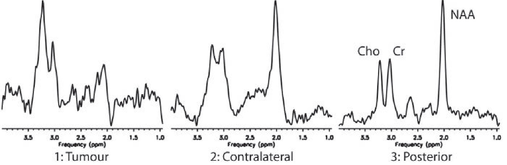
MRS metabolite ratios and clinical cut-offs

Ratio	Normal	Tumor (high-grade)	Clinical use
Cho/Cr	~1.0-1.2	>2.0-3.0	Tumor grade; >2.0 suspicious, >3.0 high-grade
NAA/Cr	~1.5-2.0	↓↓	Neuronal loss
Cho/NAA	<1.0	>1.0-3.0	Tumor vs normal
Lac/Cr	0 (absent)	Present	Anaerobic metabolism, necrosis

MRS patterns in key clinical conditions

Condition	NAA	Cho	Cr	Lactate	Lipid	Other
Normal brain	↑↑ dominant	Normal	Normal	Absent	Absent	-
Low-grade glioma	↓	↑	Normal	Absent	Absent	↑ mI
High-grade glioma/GBM	↓↓	↑↑	↓	Present	Present	Necrosis
Brain abscess	↓	↓	↓	Present	Present	Amino acids (succinate, acetate, alanine)
Radiation necrosis	↓↓	↓	↓	Present	↑↑	No Cho rise
Tumor recurrence	↓	↑↑	↓	±	±	Cho/Cr high
Acute infarct	↓	Normal/↓	↓	↑↑	±	Anaerobic
Hepatic encephalopathy	↓	↓	↓	-	-	↑ Gln/Glu, ↓ mI
MS lesion (active)	↓	↑	Normal	±	-	Demyelination
Alzheimer's disease	↓	↓	↓	-	-	↑ mI

Key clinical applications of MRS

Application	What MRS adds
Brain tumor grading	Cho/Cr and Cho/NAA ratios; lipid/lactate = necrosis = high grade
Tumor vs. abscess	Abscess: amino acids (succinate, acetate, alanine) - no Cho rise
Recurrence vs. radiation necrosis	Recurrence: ↑ Cho; Radiation necrosis: ↑ Lipid, ↓ Cho
Inborn errors of metabolism	Specific metabolite peaks (NAA ↑ in Canavan's, Cr absent in Cr deficiency)
Epilepsy	↓ NAA in hippocampus → lateralizes seizure focus
Dementia	NAA/Cr ratio in hippocampus; mI elevation in Alzheimer's
Prostate cancer	↑ Cho, ↓ Citrate → malignant (normal prostate has high citrate)
Hepatic encephalopathy	↑ Gln+Glu, ↓ Cho, ↓ mI
Stroke (acute)	Lactate ↑ = ischemic, aerobic metabolism failure
Hyperpolarized ¹³C-pyruvate	Real-time metabolic imaging - treatment response in prostate/brain tumors

Summary Table - All Four Parameters

Parameter	Type	Derived from	What it measures	Key threshold	Primary use
Tmax	Perfusion (DSC)	Deconvolution of tissue curve with AIF	Bolus arrival delay to tissue	>6 sec = penumbra	Stroke treatment selection (RAPID)
TTP	Perfusion (DSC)	Direct signal-time curve	Time to peak signal drop (no deconvolution)	3-5 sec delay = penumbra	Simpler perfusion, older protocols
rCBV	Perfusion (DSC)	Area under concentration-time curve	Relative blood volume in tissue	>1.75 = high-grade tumor	Tumor grading, recurrence vs. necrosis
MRS	Spectroscopy	Proton NMR of tissue metabolites	Chemical composition of tissue	Cho/Cr >2, ↓NAA, Lac present	Tumor characterization, metabolic disease

Explain about GRAPPA, SENSE, ASSET, SE, TSE, TRADE OFF, GRE in detail

These are core MRI acquisition techniques and parallel imaging methods. Let me pull what the textbooks have while I build the comprehensive explanation.

Searching sources...

Finding Sources

Reading File

Finding Sources

Searching Images

MRI k-space parallel imaging GRAPPA SENSE acquisition diagram

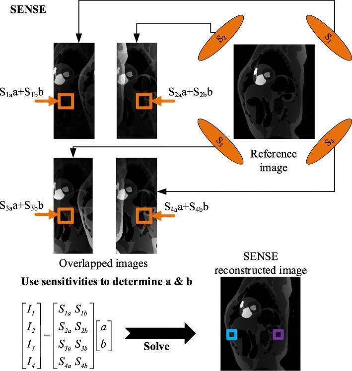
This medical image is a technical flowchart illustrating the SENSE (Sensitivity Encoding) parallel imaging reconstruction process in Magnetic Resonance Imaging (MRI). The diagram details the workflow for unfolding aliased images obtained from subsampled k-space data. It features a four-coil receiver array (represented by orange ellipses labeled S1 through S4) positioned around a reference sagittal brain image. The process begins with 'Overlapped images', which are folded sagittal MRI scans showing aliasing artifacts where multiple anatomical signals (labeled 'a' and 'b') are superimposed within each channel's view. These are mathematically represented by equations like S1a*a + S1b*b. The core of the algorithm is shown through a matrix operation that relates measured intensities (I1 to I4) to coil sensitivity values (S1a through S4b) and unknown pixel values (a, b). By solving this system of linear equations, the aliasing is resolved, resulting in the 'SENSE reconstructed image' at the bottom right. This final image demonstrates restored anatomical clarity and reduced artifacts, illustrating the clinical utility of SENSE in accelerating MRI acquisition while maintaining image integrity.

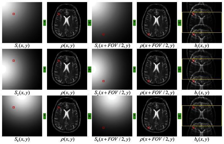
This diagnostic diagram illustrates the SENSE (Sensitivity Encoding) principles used in parallel Magnetic Resonance Imaging (MRI) reconstruction. The image is structured as a grid with three rows, representing data from the 1st, 2nd, and 8th receiver coil channels. Each row demonstrates the mathematical formulation of signal acquisition: the sensitivity map (S) for a specific pixel (x, y) is multiplied by the true brain image (ρ), then added to the sensitivity map and brain image at a location shifted by half the field of view (x + FOV/2, y). The final column shows the resulting aliased brain images (b) for each channel, characterized by overlapping anatomical structures due to k-space undersampling. The axial T2-weighted brain slices serve as the target images for reconstruction. Red square markers indicate corresponding spatial locations across the sensitivity maps and brain slices to show how two distinct spatial points alias into a single pixel in the reduced FOV acquisition. This visualization is intended for medical physics and radiology education to explain how spatial information from multiple receiver coils is used to unfold aliased images in fast MRI scanning.

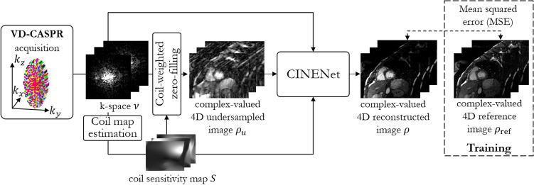
A technical flowchart illustrating the '4D CINENet' deep-learning reconstruction framework for 3D cardiac CINE MRI. The diagram begins with a VD-CASPR (Variable Density Cartesian Sampling with Poisson-Remote) k-space acquisition in the kx, ky, and kz domains. The process involves three primary parallel paths: 1) raw k-space data (ν), 2) estimation of a coil sensitivity map (S), and 3) the generation of a complex-valued 4D undersampled image (ρu) via coil-weighted zero-filling. These three elements serve as inputs to the central CINENet block. The output of the network is a complex-valued 4D reconstructed image (ρ), depicting a short-axis view of the heart. For the training phase (enclosed in a dashed box), the model applies a mean squared error (MSE) loss function to compare the reconstructed image (ρ) against a complex-valued 4D reference image (ρref), typically obtained through iterative SENSE reconstruction. This framework is designed to optimize motion-resolved cardiac imaging by mitigating undersampling artifacts.

Searching Images

spin echo gradient echo MRI sequence diagram pulse timing

A technical physics diagram illustrating the current waveforms for X (blue), Y (red), and Z (green) gradient coils in MRI pulse sequences, recorded on a Siemens Espree 1.5 T system. The top panel displays a Trufi (True Fast Imaging with Steady-state Precession) sequence characterized by trapezoidal pulses with distinct rise times, plateaus, and ramp-down phases, showing a high duty cycle and synchronous periodicity across all axes. The bottom panel shows a T2-weighted Turbo Spin Echo (T2-TSE) sequence, featuring more rectangular or square pulse shapes with rapid transitions and shorter durations compared to the Trufi sequence. These waveforms represent the electrical current sent through gradient coils to create temporary linear variations in the static magnetic field (B0) for spatial encoding of the MR signal. This comparison highlights the differences in gradient switching patterns, pulse morphology, and timing parameters between steady-state and spin-echo based sequences, which are fundamental concepts in medical imaging physics and radiology training.

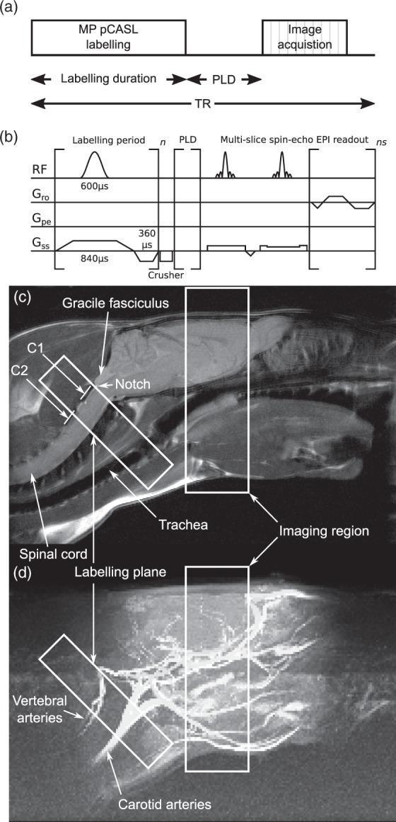
This four-panel figure illustrates a multiphase pseudo-continuous arterial spin labeling (pCASL) MRI protocol. (a) A simplified sequence schematic showing labeling duration, post-labeling delay (PLD), and acquisition within the repetition time (TR). (b) A detailed pulse timing diagram displaying radiofrequency (RF) pulses and gradient waveforms (Gro, Gpe, Gss) for labeling and multi-slice spin-echo EPI readout. (c) A sagittal fast spin-echo anatomical midline image of a Sprague Dawley rat head used for planning. Labeled landmarks include the C1 and C2 vertebrae, spinal cord, trachea, and the gracile fasciculus with a caudal notch used as a reference for placing the 6.2 mm labeling plane. (d) A maximum intensity projection of time-of-flight (TOF) angiography of the same field of view. It highlights the major neck vessels, specifically the carotid and vertebral arteries, and their orientation relative to the labeling plane and intracranial imaging region. This visual material demonstrates the methodology for optimizing labeling efficiency by aligning the labeling plane perpendicular to straight vascular segments in preclinical neuroimaging.

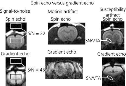
This comparison chart displays a series of magnetic resonance imaging (MRI) scans of a rodent brain, designed to demonstrate the technical differences between spin echo (SE) and gradient echo (GE) pulse sequences. The educational content is organized into three categories: Signal-to-noise (S/N), Motion artifact, and Susceptibility artifact. In the S/N comparison, the spin echo sequence shows a S/N ratio of 22, while the gradient echo sequence shows a significantly higher S/N of 45, though with increased background graininess. The motion artifact panels reveal that spin echo maintains clearer anatomical definitions, whereas the gradient echo image displays visible blurring and geometric distortion. The third section highlights susceptibility artifacts, particularly in the substantia nigra (SN) and ventral tegmental area (VTA) regions. While the spin echo sequence preserves signal in these areas, the gradient echo sequence exhibits significant signal dropout and blurring at these anatomical landmarks. This comparison serves as a clinical teaching tool for understanding pulse sequence selection in neuroimaging, emphasizing that while GE offers higher sensitivity (beneficial for fMRI and BOLD imaging), it is more prone to artifacts compared to the robust anatomical clarity of SE.

Good textbook content and excellent illustrative images found. Now delivering the comprehensive explanation:

GRAPPA, SENSE, ASSET, SE, TSE, GRE & MRI Trade-offs - Complete Guide

The Foundation: k-Space

Before explaining any sequence, you need to understand k-space - the mathematical domain where all MRI raw data lives.

k-space is a 2D grid of complex numbers
Each row of k-space = one line of frequency-encoded data, collected after one RF pulse
The center of k-space = low spatial frequencies → image contrast, brightness
The periphery of k-space = high spatial frequencies → fine detail, edges, resolution
Filling k-space completely requires many RF pulses (one per phase-encoding step)
Scanning time = TR × Number of phase-encoding lines × Number of averages

$$\text{Scan time} = TR \times N_{PE} \times NEX$$

This is why MRI is slow - you must repeat the TR cycle hundreds of times to fill k-space. All acceleration techniques aim to fill k-space faster or require fewer lines.

1. SE - Spin Echo

The fundamental MRI sequence

Spin Echo is the original and most fundamental clinical MRI pulse sequence, introduced by Hahn in 1950.

How it works - step by step

90° RF pulse → spins tip into transverse plane
       ↓
Free precession → spins begin to dephase (T2* decay)
       ↓
180° RF refocusing pulse at TE/2 → spins are rephased
       ↓
Echo forms at TE → signal is read out
       ↓
Wait for TR → longitudinal recovery (T1 relaxation)
       ↓
Repeat for next phase-encoding step

The critical element is the 180° refocusing pulse. This:

Reverses dephasing caused by local magnetic field inhomogeneities
Eliminates T2* decay (the additional signal loss from field inhomogeneities)
Leaves only true T2 decay in the echo signal

This is why SE is T2-weighted (not T2*) - field inhomogeneities are corrected out.

Parameters and weighting

TR	TE	Weighting
Short (400-700ms)	Short (10-20ms)	T1-weighted
Long (2000-4000ms)	Long (80-120ms)	T2-weighted
Long	Short	Proton density

Per Neuroanatomy through Clinical Cases: "In the spin echo (SE) pulse sequence, commonly used in clinical MRI, two time intervals are indicated: TR and TE. The choice of TR determines the time during T1 relaxation when the MRI image is obtained, while TE determines the time during T2 relaxation. A short TR (≤600ms) and short TE (≤30ms) enhance T1 contrast; a long TR (≥2000ms) and long TE (≥80ms) enhance T2 contrast."

Key properties of SE

Property	Detail
Refocusing	180° pulse corrects field inhomogeneity → no susceptibility artifact
*No T2 sensitivity**	Hemosiderin, air, metal artifacts minimized
High SAR	180° pulses deposit a lot of RF energy (specific absorption rate)
Slow	One line of k-space per TR → very long scan times
Excellent image quality	Gold standard for tissue contrast
Fat signal	Fat appears bright on T2-weighted SE (but less so than on FSE due to J-coupling effects)

Clinical limitation

A full T2-weighted brain SE at TR=3000ms with 256 phase-encoding steps and 1 NEX takes: $$3000 \times 256 \times 1 = 768,000\text{ ms} = 12.8 \text{ minutes}$$

This is impractically long → led to the development of TSE (Fast Spin Echo)

2. TSE - Turbo Spin Echo (= FSE, Fast Spin Echo)

Vendor names

Siemens: TSE (Turbo Spin Echo)
GE: FSE (Fast Spin Echo)
Philips: TSE (Turbo Spin Echo)

The revolutionary concept - Echo Train

TSE solves the speed problem of SE by collecting multiple k-space lines per TR using a train of 180° refocusing pulses:

90° → 180° → Echo 1 → 180° → Echo 2 → 180° → Echo 3 → ... → 180° → Echo N
  ←——————————— Echo Train Length (ETL) = N ———————————————→

Each echo after each 180° pulse fills a different line of k-space - all within one TR interval.

The Echo Train Length (ETL) - also called Turbo Factor

ETL = number of echoes collected per TR = number of k-space lines filled per TR

$$\text{Scan time (TSE)} = \frac{TR \times N_{PE}}{ETL} \times NEX$$

With ETL = 8, scan time is 8 times faster than conventional SE.

ETL	Speed	Trade-offs
1	Same as SE	No speed gain
4-8	4-8× faster	Some blurring
16-32	16-32× faster	More blurring, fat is brighter
Very high (HASTE/SSFSE)	Single-shot	Significant blurring

The critical concept: Effective TE

In TSE, each echo occurs at a different time point, so each echo has a different T2 decay. The effective TE is the TE of the echo that fills the center of k-space (which determines image contrast).

If the central k-space lines are filled by early echoes → short effective TE → T1/PD-weighted
If central k-space lines are filled by late echoes → long effective TE → T2-weighted

Why fat is bright on TSE T2

In conventional SE, fat loses signal on T2 due to J-coupling (spin-spin interactions between adjacent protons in fat molecules that cause T2 shortening). In TSE, the rapid 180° pulses disrupt this J-coupling → fat remains bright on T2-weighted TSE. This is why fat saturation must be added to T2-weighted TSE in most applications (e.g., liver, pelvis, breast).

Special TSE variants

Variant	ETL	Characteristic
HASTE (GE: SS-FSE)	Very high (half-Fourier single shot)	Entire k-space in one TR - fastest, blurry
BLADE / PROPELLER	Radial k-space filling	Motion-robust
Dark fluid TSE	With inversion prepulse	CSF/fluid nulled - like FLAIR
3D TSE (SPACE, CUBE, VISTA)	3D volume with high ETL	Thin isotropic slices

Comparison of Trufi (SSFP) and T2-TSE gradient waveforms - showing rectangular TSE gradient pulses vs periodic Trufi pulses, illustrating the different timing structures of these sequences

Gradient waveforms: Trufi (TruesFISP/SSFP - top) shows periodic symmetric pulses. T2-TSE (bottom) shows characteristic rectangular switching patterns of the refocusing pulse train. The structural difference in timing defines their distinct image contrast properties.

3. GRE - Gradient Echo

The key difference from SE

GRE replaces the 180° refocusing pulse with a reversed gradient to rephase transverse magnetization. This is faster and uses less RF energy but has a critical consequence: field inhomogeneities are NOT corrected.

α° RF pulse (flip angle < 90°) → transverse magnetization
       ↓
Dephasing gradient applied (negative lobe)
       ↓
Rephasing gradient applied (positive lobe, equal area) → gradient echo forms at TE
       ↓
Short TR → next pulse (before full T1 recovery)

The flip angle - the key parameter unique to GRE

GRE uses a variable flip angle (α) instead of the fixed 90° of SE:

Flip angle	Effect	Best use
Small (<30°)	Less T1 weighting, T2*-dependent	Fast imaging, MRA
Large (>60°)	More T1 weighting (Ernst angle range)	T1-weighted GRE
~Ernst angle	Maximum SNR for given TR	Optimized T1 GRE

$$\text{Ernst angle} = \cos^{-1}(e^{-TR/T1})$$

T2* instead of T2 - the critical property

Since there is no 180° refocusing pulse, GRE signal decays as T2* (T2-star), which includes:

True T2 decay (molecular interactions)
+ Additional decay from local field inhomogeneities (susceptibility effects from iron, hemosiderin, air, metal, calcification, deoxyhemoglobin)

$$\frac{1}{T2^*} = \frac{1}{T2} + \frac{1}{T2'}$$

Where T2' is the inhomogeneity component. T2* is always shorter than T2.

T2* sensitivity - clinical implications

GRE is SENSITIVE to susceptibility - areas with iron/blood/calcification/air show signal dropout:

Hemorrhage detection (hemosiderin is paramagnetic → dark spot on GRE)
Calcification (diamagnetic → dark on GRE)
Perfusion DSC uses GRE EPI (gadolinium susceptibility effect)
BOLD fMRI uses GRE (deoxyhemoglobin is paramagnetic)
SWI (Susceptibility Weighted Imaging) is a specialized GRE

MRI comparison: Spin Echo vs Gradient Echo in rat brain. SE (left) shows SNR=22, less susceptibility artifact; GRE (right) shows SNR=45, visible signal dropout at substantia nigra from iron - demonstrating T2* sensitivity and higher SNR of GRE

Direct SE vs GRE comparison. GRE gives higher SNR (45 vs 22) but shows clear susceptibility artifacts at the substantia nigra (iron-rich region) - absent on SE. Motion artifacts also visible in GRE. This is why SE is preferred for anatomical sequences and GRE for susceptibility-based applications.

GRE variants

Variant	Names	Key feature
Spoiled GRE	FLASH, SPGR, T1-FFE	Residual transverse magnetization destroyed → T1-weighted
Coherent/Refocused GRE	FISP, GRASS, FFE	Steady-state transverse magnetization maintained
SSFP	TrueFISP, FIESTA, b-FFE	Both T1 and T2 contribute - very high SNR, fluid bright
EPI	EPI	Ultra-fast GRE readout for DWI, fMRI, DSC

SE vs GRE - key comparison

Feature	Spin Echo	Gradient Echo
Refocusing pulse	180° RF pulse	Reversed gradient
Corrects field inhomogeneity	Yes	No
Decay measured	T2	T2*
SAR	High	Low
Minimum TR	Long	Very short
Speed	Slow	Fast
Susceptibility artifact	Minimal	High
Hemorrhage/iron detection	Poor	Excellent
Fat signal (T1)	Bright	Bright
Flip angle	Fixed 90°	Variable

4. Parallel Imaging - The Concept

All three techniques (GRAPPA, SENSE, ASSET) are parallel imaging methods - they use multiple receiver coil elements simultaneously to undersample k-space, then use the spatial information from coil sensitivities to reconstruct the full image.

Why parallel imaging exists

Standard MRI speed bottleneck: you must fill every line of k-space. Parallel imaging skips lines (undersamples k-space by a factor R), then reconstructs the missing data using knowledge of how each coil element "sees" the object from its position.

$$\text{Acceleration factor (R)} = \frac{\text{Lines needed without PI}}{\text{Lines actually acquired with PI}}$$

R=2 → scan is 2× faster (half the k-space lines acquired)
R=3 → 3× faster
Maximum practical R ≈ number of coil elements

Cost: SNR penalty → $SNR_{PI} \approx \frac{SNR_{full}}{g\sqrt{R}}$

Where g = geometry factor (g-factor) - a measure of coil overlap and noise amplification at each voxel. High g-factor = more noise amplification at that location.

5. SENSE - Sensitivity Encoding

Developer

Developed by Pruessmann et al. (Philips), 1999.

How SENSE works - image domain reconstruction

SENSE operates in the image domain (after Fourier transform):

Acquire sensitivity maps for each coil element (calibration scan)
Acquire undersampled k-space (every 2nd, 3rd, or Rth line skipped)
Reconstruct undersampled k-space → aliased/wrapped images (one per coil element)
Each aliased image has R copies of the FOV folded onto each other
Use the coil sensitivity maps to unfold/unwrap these aliased images mathematically

The math: For each aliased pixel pair (a, b folded together):

$$I_1 = S_{1a} \cdot a + S_{1b} \cdot b$$ $$I_2 = S_{2a} \cdot a + S_{2b} \cdot b$$

Where S = coil sensitivity, I = measured intensity in coil, a/b = unknown true pixel values.

With ≥R coil elements providing ≥R equations, solve for a and b → unfolded image.

SENSE reconstruction flowchart: 4-coil array producing aliased (folded) images for each channel, sensitivity map matrix equation, solved to produce unaliased reconstructed image

SENSE workflow: Orange ellipses = 4 receiver coil elements. Each produces an overlapped/aliased image (top center). Coil sensitivity values (S1a, S1b...) form a matrix equation. Solving the matrix for each pixel pair (a, b) produces the unfolded reconstructed image (bottom right).

SENSE aliasing mechanism: sensitivity maps × true image = aliased image per coil channel. Red squares show how two spatial locations fold onto one pixel in the reduced-FOV acquisition

SENSE mechanism: each coil (rows) produces its own aliased image (right column) where pixels from two different spatial locations (red squares) overlap. Coil sensitivity differences allow mathematical separation of these superimposed signals.

SENSE properties

Feature	Detail
Domain	Image domain (pixel unfolding)
Calibration	Pre-scan sensitivity map required
Artifact	G-factor noise amplification - central artifacts
Requirement	Reduced FOV must cover object (no wrap from anatomy)
Vendor name	Philips: SENSE; GE: ASSET (uses SENSE math); Siemens: mSENSE

6. GRAPPA - Generalized Autocalibrating Partial Parallel Acquisition

Developer

Developed by Griswold et al. (Siemens), 2002.

How GRAPPA works - k-space domain reconstruction

GRAPPA operates in k-space (before Fourier transform):

Auto-calibration lines (ACS) - a small number of fully sampled central k-space lines are acquired (these are the calibration data, not a separate scan)
The rest of k-space is undersampled (every Rth line acquired)
Use ACS data to calculate reconstruction kernels - weights that describe how missing k-space lines can be predicted from acquired lines
Apply kernels to reconstruct/synthesize missing k-space lines
Reconstruct the now-complete k-space with standard Fourier transform

The kernel is a small pattern (e.g., 3×5 block of k-space points) that learns the relationship between acquired and missing lines from the ACS data. This is done separately for each coil.

Key advantages over SENSE

Feature	GRAPPA	SENSE
Domain	k-space	Image domain
Calibration	Embedded in scan (ACS lines)	Separate sensitivity map scan needed
Robustness to motion	Better (no external calibration mismatch)	More susceptible to calibration motion
Works with partial FOV	Yes	No (object must fit reduced FOV)
Noise pattern	More uniform	Can have central g-factor peaks
Vendor	Siemens: GRAPPA; GE: ARC; Philips: CLEAR	Philips: SENSE; GE: ASSET; Siemens: mSENSE

7. ASSET - Array Spatial Sensitivity Encoding Technique

What is ASSET?

ASSET is GE Healthcare's implementation of parallel imaging, mathematically equivalent to SENSE. It uses sensitivity encoding in the image domain.

Stands for: Array Spatial Sensitivity Encoding Technique
Uses coil sensitivity profiles from a pre-scan to unfold aliased images
Available on GE MRI systems as the primary parallel imaging option
R factors typically used: 2-4 in clinical practice

ASSET vs SENSE vs GRAPPA - vendor summary

Vendor	Image-domain PI	k-space PI
Philips	SENSE	-
GE	ASSET (SENSE-type)	ARC (GRAPPA-type)
Siemens	mSENSE	GRAPPA
Canon	SPEEDER	-

All achieve the same goal (accelerated acquisition), differ in:

Whether calibration is separate or embedded
Whether reconstruction happens in image or k-space domain
Exact noise distribution and artifact patterns

Clinical use of parallel imaging (all three)

Application	Benefit
Routine brain MRI	R=2: halves scan time with acceptable SNR
Cardiac MRI	R=2-3: fit study into breath-hold window
Dynamic contrast studies (DCE, DSC)	Faster temporal resolution
High-resolution 3D studies	Feasible scan time for thin isotropic volumes
MRSI / spectroscopy	Speed improvement for metabolite maps
Combining with TSE	Very fast T2-weighted imaging

8. The Trade-offs in MRI - The Master Table

Every MRI parameter change involves a compromise between four competing goals:

           RESOLUTION
               ↑
               |
SCAN TIME ←————+————→ SNR
               |
               ↓
           COVERAGE

You can never optimize all simultaneously. This is the fundamental MRI physics constraint.

The Complete Trade-off Matrix

Parameter change	SNR	Resolution	Scan time	Artifacts	Coverage
↑ Matrix (e.g., 256→512)	↓	↑	↑	-	Same
↓ FOV	↓	↑	Same	Wrap (aliasing)	↓
↑ Slice thickness	↑	↓ (z)	Same	-	Same
↑ NEX/averages	↑ (√NEX)	Same	↑↑	↓ motion	Same
↑ TR	↑ (less T1 sat)	Same	↑↑	-	↑ slices
↓ TE	↑	Same	Same	↓ T2*	-
↑ BW (bandwidth)	↓	Same	↓ scan/line	↓ chem shift	Same
↓ BW	↑	Same	↑ scan/line	↑ chem shift	Same
↑ ETL (TSE)	↓ (blur)	↓ blur	↓↓	↑ blurring	↑ slices
Parallel imaging (R=2)	↓ (÷√2)	Same	↓ (÷R)	g-factor	Same
↑ Field strength (3T)	↑↑	Same	↓ (need less NEX)	↑ susceptibility	Same

The three fundamental trade-off triangles

Triangle 1 - Resolution vs SNR vs Scan time:

High resolution → small voxels → low SNR → must add averages → longer scan
Can't have all three optimal simultaneously

Triangle 2 - Speed vs SNR vs Coverage:

Faster scan (short TR) → less T1 recovery → lower SNR
Short TR → fewer slices possible (less time for multislice interleaving)

Triangle 3 - Parallel imaging trade-off:

Parallel imaging gives speed but costs SNR (factor of √R)
Higher acceleration (R) = faster but noisier
At very high R, g-factor noise amplification makes images clinically unusable

Practical trade-off decisions in clinical protocols

Clinical need	Trade-off made
Detect small lesion	↑ Matrix (better resolution) → accept ↓ SNR + longer time
Uncooperative patient	↓ Scan time (↓ ETL, ↑ PI) → accept ↓ SNR
Whole-spine coverage	↑ Slice number → accept ↑ TR + ↑ scan time
Fat suppression needed	Add STIR or fat-sat → accept ↓ SNR + slightly ↑ time
Better SNR in obese patient	↑ Slice thickness → accept ↓ z-resolution
Faster cardiac imaging	↑ PI (R=2-3) + ↑ bandwidth → accept ↓ SNR

9. Complete Summary - All Techniques

Technique	Type	Key mechanism	Clinical role
SE	Pulse sequence	90°→180° echo, corrects inhomogeneity	Gold standard T1/T2, no susceptibility artifact
TSE/FSE	SE variant	Multiple 180° echoes per TR (ETL)	Standard clinical T2 - fast, bright fat
GRE	Pulse sequence	Variable flip angle, gradient rephasing, T2* sensitive	T1 dynamic, hemorrhage (SWI), BOLD, DSC
GRAPPA	Parallel imaging (k-space)	ACS calibration, kernel-based k-space synthesis	Siemens primary PI; motion-robust; embedded calibration
SENSE	Parallel imaging (image domain)	Sensitivity maps, pixel unfolding algebra	Philips primary PI; simple but needs separate calibration
ASSET	Parallel imaging (image domain)	SENSE-equivalent method	GE implementation; used with all GE sequences
Trade-offs	Fundamental principle	Resolution ↔ SNR ↔ Time ↔ Coverage	Every protocol = a set of negotiated compromises

Quick Clinical Memory Rules

SE   → 180° pulse → corrects T2* → CLEAN anatomy, NO susceptibility
GRE  → gradient rephasing → T2* sensitive → BLOOD, IRON, fMRI
TSE  → multi-echo per TR (ETL) → FAST → but fat bright, slight blurring

GRAPPA → k-space reconstruction → SIEMENS → motion-robust, embedded ACS
SENSE  → image unfolding → PHILIPS → clean but needs separate sensitivity map
ASSET  → SENSE on GE machines → same math, different vendor name

Trade-offs: Resolution ↑ = SNR ↓ or Time ↑
            Speed ↑ (PI) = SNR ↓ (by √R)
            Always 3 competing: Resolution, SNR, Scan Time

Create a reference PDF summarizing MRI sequences, parameters, and clinical uses

Reading File

Running Command

mkdir -p /tmp/workspace/mri-reference && ls /tmp/workspace/

Writing File

~/mri-reference/build_mri_pdf.py

from reportlab.lib.pagesizes import A4
from reportlab.lib import colors
from reportlab.lib.styles import getSampleStyleSheet, ParagraphStyle
from reportlab.lib.units import mm, cm
from reportlab.platypus import (
    SimpleDocTemplate, Paragraph, Spacer, Table, TableStyle,
    HRFlowable, PageBreak, KeepTogether
)
from reportlab.lib.enums import TA_CENTER, TA_LEFT, TA_JUSTIFY
from reportlab.platypus import BaseDocTemplate, Frame, PageTemplate
from reportlab.lib.colors import HexColor

OUTPUT = "/tmp/workspace/mri-reference/MRI_Reference_Guide.pdf"

# ── Colour palette ──────────────────────────────────────────────────────────
NAVY      = HexColor("#1a3a5c")
TEAL      = HexColor("#0d7377")
LIGHT_TEAL= HexColor("#e8f7f8")
MID_TEAL  = HexColor("#b2e0e3")
ORANGE    = HexColor("#e07b39")
LIGHT_ORANGE = HexColor("#fdf0e8")
GREY_BG   = HexColor("#f4f6f8")
DARK_GREY = HexColor("#444444")
TABLE_HDR = HexColor("#1a3a5c")
TABLE_ALT = HexColor("#eef4f7")
WHITE     = colors.white
BLACK     = colors.black

# ── Page setup ──────────────────────────────────────────────────────────────
PAGE_W, PAGE_H = A4
MARGIN = 18*mm

def header_footer(canvas, doc):
    canvas.saveState()
    # Header bar
    canvas.setFillColor(NAVY)
    canvas.rect(0, PAGE_H - 22*mm, PAGE_W, 22*mm, fill=1, stroke=0)
    canvas.setFillColor(WHITE)
    canvas.setFont("Helvetica-Bold", 11)
    canvas.drawString(MARGIN, PAGE_H - 14*mm, "MRI Sequences, Parameters & Clinical Uses")
    canvas.setFont("Helvetica", 9)
    canvas.drawRightString(PAGE_W - MARGIN, PAGE_H - 14*mm, "Quick Reference Guide")
    # Footer
    canvas.setFillColor(NAVY)
    canvas.rect(0, 0, PAGE_W, 12*mm, fill=1, stroke=0)
    canvas.setFillColor(WHITE)
    canvas.setFont("Helvetica", 8)
    canvas.drawString(MARGIN, 4*mm, "MRI Physics & Clinical Reference  |  Orris Medical AI")
    canvas.drawRightString(PAGE_W - MARGIN, 4*mm, f"Page {doc.page}")
    canvas.restoreState()

doc = SimpleDocTemplate(
    OUTPUT,
    pagesize=A4,
    leftMargin=MARGIN, rightMargin=MARGIN,
    topMargin=26*mm, bottomMargin=16*mm,
    title="MRI Sequences, Parameters & Clinical Uses",
    author="Orris Medical AI",
    subject="MRI Quick Reference Guide"
)

# ── Styles ──────────────────────────────────────────────────────────────────
styles = getSampleStyleSheet()

def S(name, **kw):
    return ParagraphStyle(name, **kw)

H1 = S("H1", fontSize=18, textColor=WHITE, fontName="Helvetica-Bold",
        alignment=TA_CENTER, spaceAfter=4)
H2 = S("H2", fontSize=13, textColor=WHITE, fontName="Helvetica-Bold",
        alignment=TA_LEFT, spaceAfter=2, spaceBefore=2)
H3 = S("H3", fontSize=10, textColor=NAVY, fontName="Helvetica-Bold",
        spaceAfter=3, spaceBefore=6)
BODY = S("BODY", fontSize=8.5, textColor=DARK_GREY, fontName="Helvetica",
         leading=13, spaceAfter=4, alignment=TA_JUSTIFY)
SMALL = S("SMALL", fontSize=7.5, textColor=DARK_GREY, fontName="Helvetica",
          leading=11, spaceAfter=2)
BULLET = S("BULLET", fontSize=8.5, textColor=DARK_GREY, fontName="Helvetica",
           leading=13, leftIndent=12, spaceAfter=2,
           bulletIndent=4, bulletText="•")
CAPTION = S("CAPTION", fontSize=7.5, textColor=HexColor("#666666"),
            fontName="Helvetica-Oblique", alignment=TA_CENTER, spaceAfter=4)
TBL_H = S("TBL_H", fontSize=8, textColor=WHITE, fontName="Helvetica-Bold",
          alignment=TA_CENTER)
TBL_C = S("TBL_C", fontSize=7.5, textColor=DARK_GREY, fontName="Helvetica",
          alignment=TA_LEFT, leading=11)
TBL_CC = S("TBL_CC", fontSize=7.5, textColor=DARK_GREY, fontName="Helvetica",
           alignment=TA_CENTER, leading=11)

def section_banner(text, color=NAVY):
    data = [[Paragraph(text, H2)]]
    t = Table(data, colWidths=[PAGE_W - 2*MARGIN])
    t.setStyle(TableStyle([
        ("BACKGROUND", (0,0), (-1,-1), color),
        ("TOPPADDING",  (0,0), (-1,-1), 5),
        ("BOTTOMPADDING",(0,0),(-1,-1), 5),
        ("LEFTPADDING", (0,0), (-1,-1), 8),
    ]))
    return t

def sub_banner(text):
    data = [[Paragraph(text, S("SB", fontSize=9, textColor=NAVY,
                               fontName="Helvetica-Bold", spaceAfter=0))]]
    t = Table(data, colWidths=[PAGE_W - 2*MARGIN])
    t.setStyle(TableStyle([
        ("BACKGROUND", (0,0), (-1,-1), LIGHT_TEAL),
        ("TOPPADDING",  (0,0), (-1,-1), 4),
        ("BOTTOMPADDING",(0,0),(-1,-1), 4),
        ("LEFTPADDING", (0,0), (-1,-1), 8),
        ("LINEBELOW", (0,0), (-1,-1), 0.5, TEAL),
    ]))
    return t

def make_table(headers, rows, col_widths=None, alt=True):
    cw = col_widths or [PAGE_W/len(headers) - 2*MARGIN/(len(headers))] * len(headers)
    data = [[Paragraph(h, TBL_H) for h in headers]]
    for i, row in enumerate(rows):
        data.append([Paragraph(str(c), TBL_C) for c in row])
    ts = TableStyle([
        ("BACKGROUND",   (0,0), (-1,0),  TABLE_HDR),
        ("ROWBACKGROUNDS",(0,1),(-1,-1), [WHITE, TABLE_ALT] if alt else [WHITE]),
        ("GRID",         (0,0), (-1,-1), 0.3, HexColor("#cccccc")),
        ("VALIGN",       (0,0), (-1,-1), "TOP"),
        ("TOPPADDING",   (0,0), (-1,-1), 4),
        ("BOTTOMPADDING",(0,0), (-1,-1), 4),
        ("LEFTPADDING",  (0,0), (-1,-1), 5),
        ("RIGHTPADDING", (0,0), (-1,-1), 5),
    ])
    t = Table(data, colWidths=cw, repeatRows=1)
    t.setStyle(ts)
    return t

def info_box(text, bg=LIGHT_TEAL, border=TEAL):
    data = [[Paragraph(text, SMALL)]]
    t = Table(data, colWidths=[PAGE_W - 2*MARGIN])
    t.setStyle(TableStyle([
        ("BACKGROUND",  (0,0),(-1,-1), bg),
        ("LINEAFTER",   (0,0),(0,-1),  2, border),
        ("LINEBEFORE",  (0,0),(0,-1),  2, border),
        ("TOPPADDING",  (0,0),(-1,-1), 6),
        ("BOTTOMPADDING",(0,0),(-1,-1),6),
        ("LEFTPADDING", (0,0),(-1,-1), 8),
    ]))
    return t

# ── Content ──────────────────────────────────────────────────────────────────
story = []
SP = lambda n=6: Spacer(1, n)

# ══════════════════════════════════════════════════════════════════════
#  TITLE PAGE
# ══════════════════════════════════════════════════════════════════════
# Big title banner
title_data = [[Paragraph("MRI Sequences, Parameters<br/>&amp; Clinical Uses", 
                          S("TP", fontSize=22, textColor=WHITE, fontName="Helvetica-Bold",
                            alignment=TA_CENTER, leading=30))]]
title_tbl = Table(title_data, colWidths=[PAGE_W - 2*MARGIN])
title_tbl.setStyle(TableStyle([
    ("BACKGROUND",   (0,0),(-1,-1), NAVY),
    ("TOPPADDING",   (0,0),(-1,-1), 18),
    ("BOTTOMPADDING",(0,0),(-1,-1), 18),
]))
story.append(title_tbl)
story.append(SP(8))

subtitle_data = [[Paragraph("Quick Reference Guide for Radiographers, Radiologists &amp; Clinicians",
                              S("ST", fontSize=11, textColor=TEAL, fontName="Helvetica-Bold",
                                alignment=TA_CENTER))]]
st = Table(subtitle_data, colWidths=[PAGE_W - 2*MARGIN])
st.setStyle(TableStyle([("TOPPADDING",(0,0),(-1,-1),4),("BOTTOMPADDING",(0,0),(-1,-1),4)]))
story.append(st)
story.append(SP(6))
story.append(HRFlowable(width="100%", thickness=1.5, color=TEAL))
story.append(SP(6))

# Contents overview box
toc_items = [
    "1. MRI Fundamentals — TR, TE, TI, Flip Angle",
    "2. Core Sequences — T1, T2, FLAIR, STIR, CISS",
    "3. Pulse Sequence Types — SE, TSE/FSE, GRE",
    "4. Signal Characteristics — Quick Identification Tables",
    "5. Advanced Diffusion — DWI, ADC, DTI",
    "6. Perfusion Imaging — DSC, DCE, ASL",
    "7. Perfusion Parameters — Tmax, TTP, rCBV",
    "8. MR Spectroscopy (MRS) — Metabolites & Patterns",
    "9. Parallel Imaging — GRAPPA, SENSE, ASSET",
    "10. SNR, CNR & Bandwidth",
    "11. MRI Trade-offs — The Master Table",
    "12. Clinical Protocol Guide",
]
toc_text = "<b>Contents</b><br/><br/>" + "<br/>".join(toc_items)
story.append(info_box(toc_text, bg=GREY_BG, border=NAVY))
story.append(SP(8))
story.append(Paragraph("Compiled from: Grainger &amp; Allison's Diagnostic Radiology · Cummings Otolaryngology · "
                        "Bradley &amp; Daroff's Neurology · Harrison's Principles of Internal Medicine · "
                        "Washington Manual of Medical Therapeutics",
                        CAPTION))
story.append(PageBreak())

# ══════════════════════════════════════════════════════════════════════
#  SECTION 1 — MRI FUNDAMENTALS
# ══════════════════════════════════════════════════════════════════════
story.append(section_banner("1.  MRI FUNDAMENTALS — TR, TE, TI & Flip Angle"))
story.append(SP(6))

story.append(Paragraph(
    "MRI signal arises from hydrogen protons aligning in a magnetic field, being perturbed by RF pulses, "
    "then emitting energy as they return to equilibrium. Three timing parameters define image contrast:",
    BODY))
story.append(SP(4))

params_data = [
    ["Parameter", "Full Name", "Controls", "Short Value Effect", "Long Value Effect"],
    ["TR", "Repetition Time", "T1 contrast / longitudinal recovery",
     "T1-weighted (contrast between tissues with diff. T1)", "T1 saturation removed → PD/T2"],
    ["TE", "Echo Time", "T2/T2* contrast / transverse decay",
     "Minimises T2 decay → higher SNR, less T2 contrast", "More T2 decay → T2-weighted"],
    ["TI", "Inversion Time", "Tissue nulling in IR sequences",
     "Nulls short-T1 tissue (fat: ~140 ms = STIR)", "Nulls long-T1 tissue (CSF: ~2200 ms = FLAIR)"],
    ["Flip angle (α)", "RF tip angle", "T1 saturation / SNR / speed",
     "Small α: less T1, faster GRE, MRA", "Large α: more T1 weighting (T1-GRE)"],
]
story.append(make_table(
    params_data[0], params_data[1:],
    col_widths=[18*mm, 30*mm, 45*mm, 48*mm, 48*mm]
))
story.append(SP(6))

story.append(info_box(
    "<b>Key formula:</b>  Scan Time = TR × N<sub>PE</sub> × NEX  |  "
    "SNR ∝ Voxel Volume × √NEX / √BW  |  "
    "T2* = T2 + field inhomogeneity component (always shorter than T2)",
    bg=LIGHT_TEAL, border=TEAL))
story.append(PageBreak())

# ══════════════════════════════════════════════════════════════════════
#  SECTION 2 — CORE SEQUENCES
# ══════════════════════════════════════════════════════════════════════
story.append(section_banner("2.  CORE MRI SEQUENCES"))
story.append(SP(6))

seq_data = [
    ["Sequence", "TR", "TE", "TI", "Fat", "CSF", "Pathology", "Key Use"],
    ["T1-weighted","Short\n400–700ms","Short\n10–20ms","None",
     "BRIGHT","DARK","Intermediate","Anatomy, hemorrhage, Gad enhancement"],
    ["T2-weighted","Long\n2000–4000ms","Long\n50–90ms","None",
     "Intermediate","BRIGHT","BRIGHT","Lesion detection, fluid, edema"],
    ["FLAIR","Very long\n~10,000ms","Long\n~120ms","Long\n~2200ms (nulls CSF)",
     "Bright","DARK (suppressed)","BRIGHT","Periventricular lesions, MS, SAH, stroke timing"],
    ["STIR","Long","Long","Short\n~140ms (nulls fat)",
     "DARK (suppressed)","BRIGHT","Very BRIGHT","Bone marrow edema, muscle, extremities"],
    ["CISS","Very short\n5–20ms","Short","None",
     "Intermediate","Very BRIGHT","DARK (against bright CSF)","Cranial nerves, inner ear, IAC, CPA"],
    ["DWI (b=1000)","Long","Short","None",
     "Intermediate","DARK","BRIGHT if restricted","Acute stroke, abscess, hypercellular tumor"],
    ["ADC map","(derived)","(derived)","None",
     "Intermediate","BRIGHT","DARK if restricted","Confirm true restriction, remove T2 shine-through"],
]
story.append(make_table(
    seq_data[0], seq_data[1:],
    col_widths=[22*mm, 22*mm, 22*mm, 28*mm, 18*mm, 24*mm, 28*mm, 45*mm]
))
story.append(SP(6))

story.append(sub_banner("Quick Identification Rules"))
story.append(SP(4))
id_rules = [
    ("T1", "Fat = WHITE  |  CSF = BLACK  |  Subacute blood = WHITE  |  Gad-enhancing tissue = WHITE"),
    ("T2", "CSF = WHITE  |  Muscle = GREY  |  Bone/hemosiderin = BLACK  |  Pathology = usually BRIGHT"),
    ("FLAIR", "CSF = BLACK  |  White matter lesions = WHITE  |  Periventricular lesions conspicuous"),
    ("STIR", "Fat = BLACK  |  Edema/fluid/tumor = BRIGHT WHITE  |  Works at field inhomogeneous sites"),
    ("CISS", "CSF = VERY BRIGHT  |  Nerves = DARK  |  Sub-mm cranial nerve visualization"),
    ("DWI+ADC", "True restriction: DWI BRIGHT + ADC DARK  |  T2 shine-through: both bright on DWI & ADC"),
]
id_data = [["Sequence", "Rule"]] + [[r[0], r[1]] for r in id_rules]
story.append(make_table(id_data[0], id_data[1:], col_widths=[22*mm, PAGE_W - 2*MARGIN - 22*mm - 10*mm]))
story.append(PageBreak())

# ══════════════════════════════════════════════════════════════════════
#  SECTION 3 — PULSE SEQUENCE TYPES
# ══════════════════════════════════════════════════════════════════════
story.append(section_banner("3.  PULSE SEQUENCE TYPES — SE, TSE, GRE"))
story.append(SP(6))

story.append(sub_banner("Spin Echo (SE)"))
story.append(SP(3))
story.append(Paragraph(
    "The fundamental MRI sequence. Uses a 90° excitation pulse followed by a 180° refocusing pulse. "
    "The 180° pulse rephases dephased spins, eliminating T2* decay and leaving only true T2. "
    "Result: clean anatomical images with no susceptibility artifact — but slow (one k-space line per TR).",
    BODY))
story.append(SP(4))

story.append(sub_banner("Turbo Spin Echo (TSE) = Fast Spin Echo (FSE)"))
story.append(SP(3))
story.append(Paragraph(
    "Solves SE's speed problem by collecting multiple echoes (echo train, ETL) per TR using repeated "
    "180° pulses. Each echo fills a different k-space line. ETL=8 means 8× speed increase. "
    "<b>Fat is bright</b> on T2 TSE (J-coupling disrupted by rapid 180° pulses) — add fat saturation when needed. "
    "<b>Effective TE</b> = TE of the echo filling the center of k-space (determines contrast).",
    BODY))
story.append(SP(4))

story.append(sub_banner("Gradient Echo (GRE)"))
story.append(SP(3))
story.append(Paragraph(
    "Replaces the 180° refocusing pulse with a reversed gradient. <b>Field inhomogeneities are NOT corrected</b> "
    "→ signal decays as T2* (not T2). Uses a variable flip angle (α). Short TR possible → very fast. "
    "Key property: susceptibility-sensitive → detects hemorrhage, iron, calcification. "
    "Foundation for BOLD fMRI, SWI, DSC perfusion.",
    BODY))
story.append(SP(5))

se_gre_data = [
    ["Feature", "Spin Echo", "TSE / FSE", "Gradient Echo"],
    ["Refocusing", "180° RF pulse", "Multiple 180° RF pulses", "Reversed gradient"],
    ["Corrects inhomogeneity", "YES", "YES", "NO"],
    ["Decay type", "T2", "T2 (effective)", "T2*"],
    ["Speed", "Slow", "FAST (ETL×)", "Very fast"],
    ["SAR (RF energy)", "High", "Very high", "LOW"],
    ["Susceptibility artifact", "Minimal", "Minimal", "HIGH"],
    ["Hemorrhage detection", "Poor", "Poor", "EXCELLENT"],
    ["Fat on T2", "Dark (J-coupling)", "BRIGHT (J-coupling lost)", "Variable"],
    ["Flip angle", "Fixed 90°", "Fixed 90° (excitation)", "VARIABLE (α)"],
    ["SNR", "Good", "Good", "High (but T2* noise)"],
    ["Primary clinical use", "Gold standard anatomy", "Standard T2 brain/body", "Dynamic, SWI, fMRI, GRE T1"],
]
story.append(make_table(
    se_gre_data[0], se_gre_data[1:],
    col_widths=[42*mm, 43*mm, 43*mm, 45*mm]
))
story.append(SP(5))

story.append(sub_banner("GRE Variants"))
story.append(SP(3))
gre_var_data = [
    ["Variant", "Siemens", "GE", "Philips", "Characteristic"],
    ["Spoiled GRE", "FLASH", "SPGR", "T1-FFE", "T1-weighted — residual transverse magnetization destroyed"],
    ["Coherent GRE", "FISP", "GRASS", "FFE", "Steady-state — T1/T2* contrast"],
    ["SSFP (balanced)", "TrueFISP", "FIESTA", "b-FFE", "Very high SNR — fluid bright — cardiac, MSK"],
    ["EPI", "EPI", "EPI", "EPI", "Ultra-fast GRE readout — DWI, fMRI, DSC perfusion"],
    ["SWI", "SWI", "SWAN", "Venous BOLD", "3D GRE — phase + magnitude — microhemorrhage, iron"],
]
story.append(make_table(
    gre_var_data[0], gre_var_data[1:],
    col_widths=[30*mm, 20*mm, 20*mm, 22*mm, 81*mm]
))
story.append(PageBreak())

# ══════════════════════════════════════════════════════════════════════
#  SECTION 4 — CLINICAL APPLICATIONS
# ══════════════════════════════════════════════════════════════════════
story.append(section_banner("4.  CLINICAL APPLICATIONS BY ANATOMY"))
story.append(SP(6))

story.append(sub_banner("Brain MRI — Standard Protocol"))
story.append(SP(3))
brain_data = [
    ["Sequence", "Plane", "Purpose"],
    ["T2 TSE", "Axial", "Lesion detection — tumor, edema, demyelination, infarct"],
    ["FLAIR", "Axial", "White matter lesions, periventricular plaques, SAH, cortical lesions"],
    ["T1 SE/GRE", "Axial", "Anatomy, hemorrhage staging, bone marrow"],
    ["DWI + ADC", "Axial", "Acute stroke (minutes), abscess, hypercellular tumor, CJD"],
    ["T1 + Gadolinium", "Axial/Cor/Sag", "Blood-brain barrier breakdown — tumor, infection, MS, leptomeningeal"],
    ["CISS 3D", "Axial/Coronal", "IAC, cranial nerves, CPA angle, inner ear"],
    ["SWI", "Axial", "Microhemorrhage, DVA, cavernoma, venous sinus, amyloid angiopathy"],
    ["MRS", "VOI selection", "Metabolite profiling — tumor grading, recurrence vs necrosis"],
    ["DSC perfusion", "Axial", "rCBV for tumor grading; penumbra in stroke"],
]
story.append(make_table(brain_data[0], brain_data[1:],
    col_widths=[38*mm, 30*mm, PAGE_W - 2*MARGIN - 68*mm - 10*mm]))
story.append(SP(5))

story.append(sub_banner("Spine MRI — Standard Protocol"))
story.append(SP(3))
spine_data = [
    ["Sequence", "Plane", "Purpose"],
    ["T1 SE", "Sagittal", "Anatomy, cord signal, bone marrow (infiltration = dark), disc height"],
    ["T2 TSE", "Sagittal", "CSF (bright), disc hydration, cord edema/myelopathy"],
    ["STIR", "Sagittal", "Cord/marrow edema, ligament injury, metastases, fracture"],
    ["T2 TSE", "Axial", "Disc herniation, nerve root compression, foraminal stenosis"],
    ["T1 + Gadolinium", "Sagittal + Axial", "Leptomeningeal, epidural abscess, cord tumor enhancement"],
]
story.append(make_table(spine_data[0], spine_data[1:],
    col_widths=[38*mm, 30*mm, PAGE_W - 2*MARGIN - 68*mm - 10*mm]))
story.append(SP(5))

story.append(sub_banner("Abdomen/Liver MRI"))
story.append(SP(3))
liver_data = [
    ["Sequence", "Purpose"],
    ["T2 TSE (respiratory triggered)", "Cyst vs solid — hemangioma very bright ('light bulb' sign)"],
    ["T1 GRE in/out of phase", "Fat quantification — steatosis, lipid in adrenal adenoma"],
    ["T1 GRE + Gadolinium (multiphase)", "Arterial, portal venous, delayed phases — HCC, FNH, adenoma"],
    ["DWI + ADC", "Restricted diffusion in HCC, abscess, cholangiocarcinoma, mets"],
    ["MRCP (heavily T2-weighted)", "Biliary tree, pancreatic duct — non-invasive ERCP alternative"],
    ["DCE MRI", "Ktrans permeability mapping for treatment response"],
]
story.append(make_table(liver_data[0], liver_data[1:],
    col_widths=[55*mm, PAGE_W - 2*MARGIN - 55*mm - 10*mm]))
story.append(PageBreak())

# ══════════════════════════════════════════════════════════════════════
#  SECTION 5 — DWI & DTI
# ══════════════════════════════════════════════════════════════════════
story.append(section_banner("5.  DIFFUSION IMAGING — DWI, ADC & DTI"))
story.append(SP(6))

story.append(sub_banner("DWI Physics"))
story.append(SP(3))
story.append(Paragraph(
    "DWI applies paired diffusion-sensitizing gradients either side of the 180° refocusing pulse. "
    "Moving water molecules dephase (signal LOSS). Restricted molecules stay in phase (signal PRESERVED = BRIGHT). "
    "<b>b-value</b> controls sensitivity — clinical standard b=1000 s/mm². "
    "<b>ADC map</b> = quantitative diffusion rate derived from ≥2 b-values, eliminates T2 shine-through.",
    BODY))
story.append(SP(4))

story.append(Paragraph("<b>True Restriction Rule:  DWI BRIGHT + ADC DARK</b>  (T2 shine-through = both bright)", 
                       S("RULE", fontSize=9, textColor=NAVY, fontName="Helvetica-Bold",
                         spaceAfter=6, leftIndent=10)))

dwi_data = [
    ["Condition", "DWI", "ADC", "Mechanism"],
    ["Acute ischemic stroke", "BRIGHT", "DARK", "Cytotoxic edema — Na/K pump failure → cell swelling"],
    ["Brain abscess (center)", "BRIGHT", "DARK", "Viscous pus — proteins restrict water movement"],
    ["Epidermoid cyst", "BRIGHT", "DARK", "Keratin debris — restricted motion (vs arachnoid: free)"],
    ["CNS lymphoma", "BRIGHT", "DARK", "Hypercellular — packed cells restrict extracellular diffusion"],
    ["GBM (cellular zones)", "Bright", "Dark", "High cellularity in solid tumor parts"],
    ["Creutzfeldt-Jakob (CJD)", "BRIGHT", "DARK", "Cortical ribboning + basal ganglia — prion-related"],
    ["Diffuse axonal injury", "Bright", "Dark", "Shear injury at grey-white junction, corpus callosum"],
    ["Simple cyst", "Dark", "BRIGHT", "Free water — high ADC (no restriction)"],
    ["T2 shine-through", "Bright", "Normal/Bright", "Long T2 artefact — NOT true restriction"],
    ["Post-treatment necrosis", "Dark/variable", "High", "Cell death — freed water, increased ADC"],
]
story.append(make_table(dwi_data[0], dwi_data[1:],
    col_widths=[42*mm, 18*mm, 16*mm, PAGE_W - 2*MARGIN - 76*mm - 10*mm]))
story.append(SP(5))

story.append(sub_banner("DWI-FLAIR Mismatch (Stroke)"))
story.append(SP(3))
story.append(Paragraph(
    "<b>DWI bright + FLAIR negative</b> = stroke onset &lt;4.5–6 hours → tissue may be salvageable → "
    "consider thrombolysis/thrombectomy even if onset time unknown.<br/>"
    "<b>DWI bright + FLAIR bright</b> = stroke likely &gt;6 hours → beyond conventional thrombolysis window.",
    BODY))
story.append(SP(5))

story.append(sub_banner("DTI — Diffusion Tensor Imaging"))
story.append(SP(3))
story.append(Paragraph(
    "DTI measures diffusion in ≥6 directions to characterize the 3D diffusion ellipsoid at each voxel. "
    "In white matter, diffusion is <b>anisotropic</b> (moves freely along axons, restricted across). "
    "Tractography reconstructs white matter fiber tracts for surgical planning.",
    BODY))
story.append(SP(4))

dti_data = [
    ["DTI Metric", "What it measures", "Normal WM", "Abnormal finding"],
    ["FA (Fractional Anisotropy)", "Directionality of diffusion (0=sphere, 1=line)", "0.3–0.8", "↓ FA = damaged/infiltrated white matter"],
    ["MD (Mean Diffusivity)", "Average diffusion rate in all directions", "~0.8×10⁻³", "↑ MD = tissue destruction/edema"],
    ["Axial Diffusivity (AD)", "Diffusion along principal axis (along axon)", "High", "↓ AD = axonal injury"],
    ["Radial Diffusivity (RD)", "Diffusion perpendicular to axon", "Low", "↑ RD = demyelination"],
]
story.append(make_table(dti_data[0], dti_data[1:],
    col_widths=[45*mm, 58*mm, 25*mm, 55*mm]))

story.append(SP(4))
dti_use_data = [
    ["Clinical Use", "Detail"],
    ["Pre-operative brain tumor", "Map corticospinal tract, arcuate fasciculus relative to tumor — guide safe resection"],
    ["TBI / Diffuse axonal injury", "↓ FA in WM tracts even when conventional MRI normal"],
    ["Multiple sclerosis", "↓ FA in normal-appearing WM — progression biomarker"],
    ["Epilepsy pre-surgery", "Map optic radiations before temporal lobectomy to preserve vision"],
    ["Stroke prognosis", "Wallerian degeneration of corticospinal tract — low FA predicts poor motor recovery"],
    ["Tractography colors", "Red = L-R (corpus callosum) | Green = A-P (cingulum, uncinate) | Blue = S-I (CST, IC)"],
]
story.append(make_table(dti_use_data[0], dti_use_data[1:],
    col_widths=[55*mm, PAGE_W - 2*MARGIN - 55*mm - 10*mm]))
story.append(PageBreak())

# ══════════════════════════════════════════════════════════════════════
#  SECTION 6 — PERFUSION IMAGING
# ══════════════════════════════════════════════════════════════════════
story.append(section_banner("6.  PERFUSION IMAGING — DSC, DCE & ASL"))
story.append(SP(6))

perf_compare = [
    ["Feature", "DSC", "DCE", "ASL"],
    ["Contrast agent", "Gadolinium (required)", "Gadolinium (required)", "NONE (magnetic labeling)"],
    ["MRI sequence", "T2* GRE EPI", "T1 spoiled GRE", "EPI (subtraction)"],
    ["Mechanism", "Susceptibility → signal LOSS", "T1 shortening → signal GAIN", "Inverted blood water subtraction"],
    ["BBB assumption", "Intact (or leakage-corrected)", "Disruption is measured", "Not applicable"],
    ["Primary outputs", "CBV, CBF, MTT, Tmax, TTP", "Ktrans, ve, vp, IAUC", "Absolute CBF (mL/100g/min)"],
    ["Time resolution", "~1–2 sec (fast)", "~5–10 sec (moderate)", "3–5 min total (averaged)"],
    ["SNR", "High", "High", "LOW (0.5–1.5% signal)"],
    ["Contraindication", "Renal failure, Gd allergy", "Renal failure, Gd allergy", "NONE"],
    ["Best brain use", "Stroke penumbra, rCBV", "Tumor permeability/response", "Pediatric, dementia, CKD"],
    ["Body use", "Limited", "Prostate, breast, cervix", "Limited"],
    ["Quantitative?", "Semi (rCBV relative)", "Yes (Ktrans min⁻¹)", "Yes (absolute CBF)"],
]
story.append(make_table(perf_compare[0], perf_compare[1:],
    col_widths=[42*mm, 53*mm, 50*mm, 48*mm]))
story.append(SP(6))

story.append(sub_banner("DSC Perfusion — Derived Parameters"))
story.append(SP(3))
dsc_params = [
    ["Parameter", "Full Name", "Unit", "Measures", "Ischemia finding"],
    ["CBV", "Cerebral Blood Volume", "mL/100g", "Volume of blood in tissue", "↓ in core (↑ in oligaemia by autoregulation)"],
    ["CBF", "Cerebral Blood Flow", "mL/100g/min", "Flow through tissue per minute", "↓↓ in core, ↓ in penumbra"],
    ["MTT", "Mean Transit Time", "seconds", "Avg time for blood to cross capillary bed", "↑ in penumbra and core"],
    ["Tmax", "Time to max of residue fn", "seconds", "Bolus arrival delay at tissue", "↑ → >6s = penumbra"],
    ["TTP", "Time to Peak signal drop", "seconds", "Time to peak contrast in voxel", "↑ by 3–5s = penumbra"],
    ["rCBV", "Relative CBV (tumors)", "ratio vs WM", "Blood volume relative to normal WM", ">1.75 = high-grade tumor"],
]
story.append(make_table(dsc_params[0], dsc_params[1:],
    col_widths=[20*mm, 40*mm, 18*mm, 45*mm, 50*mm]))
story.append(SP(4))

story.append(info_box(
    "<b>Stroke penumbra rule:</b>  Tmax &gt;6s = penumbra  |  DWI = infarct core  |  "
    "Mismatch (Tmax&gt;6s vol / DWI vol) ≥1.2 AND ≥15 mL → favorable for thrombectomy (DAWN/DEFUSE-3 criteria)<br/>"
    "<b>Tumor rCBV:</b>  &gt;1.75 = high-grade glioma  |  Low rCBV + enhancing lesion = radiation necrosis  |  "
    "High rCBV + enhancing lesion = tumor recurrence",
    bg=LIGHT_ORANGE, border=ORANGE))
story.append(SP(4))

story.append(sub_banner("DCE Pharmacokinetic Parameters (Tofts Model)"))
story.append(SP(3))
dce_data = [
    ["Parameter", "Symbol", "Unit", "Meaning", "Clinical interpretation"],
    ["Volume transfer constant", "Ktrans", "min⁻¹", "Rate of Gd transfer from plasma to EES (permeability × surface area)",
     "↑ in high-grade glioma, metastases, active MS. ↓ with anti-angiogenic therapy"],
    ["EES volume fraction", "ve", "fraction", "Fraction of tissue that is extravascular extracellular space",
     "Related to tumor cellularity"],
    ["Plasma volume fraction", "vp", "fraction", "Fractional blood plasma volume in tissue",
     "Reflects vascularity"],
    ["Washout rate constant", "kep=Ktrans/ve", "min⁻¹", "Rate of Gd transfer back from EES to plasma",
     "Kinetic curve shape (washout pattern)"],
    ["Initial area under curve", "IAUC", "mmol·min/L", "Gd uptake in first 60s",
     "Empirical fast perfusion metric — used in breast, prostate"],
]
story.append(make_table(dce_data[0], dce_data[1:],
    col_widths=[35*mm, 16*mm, 16*mm, 52*mm, 54*mm]))
story.append(PageBreak())

# ══════════════════════════════════════════════════════════════════════
#  SECTION 7 — MR SPECTROSCOPY
# ══════════════════════════════════════════════════════════════════════
story.append(section_banner("7.  MR SPECTROSCOPY (MRS)"))
story.append(SP(6))

story.append(Paragraph(
    "MRS detects NMR signals from tissue metabolites. Each molecule's hydrogen nuclei resonate at a slightly "
    "different frequency (chemical shift, in ppm), producing a characteristic spectrum. "
    "The area under each peak ∝ metabolite concentration. Used at 1.5T and 3T; single-voxel (SVS) or "
    "multi-voxel (MRSI/CSI) acquisition.",
    BODY))
story.append(SP(5))

story.append(sub_banner("Key Brain Metabolites"))
story.append(SP(3))
met_data = [
    ["Metabolite", "Abbrev.", "ppm", "Source", "↑ means", "↓ means"],
    ["N-Acetylaspartate", "NAA", "2.0", "Neurons only", "Neuronal recovery (rare)", "Neuronal loss/death — stroke, tumor, atrophy"],
    ["Choline", "Cho", "3.2", "Cell membrane turnover", "Tumor, demyelination, proliferation", "Necrosis, hepatic encephalopathy"],
    ["Creatine", "Cr", "3.0", "Energy metabolism", "—", "Necrosis; used as stable internal reference"],
    ["Lactate", "Lac", "1.33", "Anaerobic glycolysis", "Ischemia, necrosis, high-grade tumor", "Normal (absent in healthy brain)"],
    ["Lipids", "Lip", "0.9–1.3", "Free (released from membranes)", "Necrosis, GBM, abscess", "Normal (undetectable in healthy brain)"],
    ["Myo-inositol", "mI", "3.56", "Astrocytes (short TE only)", "Low-grade glioma, Alzheimer's", "Hepatic encephalopathy"],
    ["Glutamate/Glutamine", "Glx", "2.1–2.5", "Neurotransmission", "Hyperammonemia, hepatic encephalopathy", "—"],
]
story.append(make_table(met_data[0], met_data[1:],
    col_widths=[35*mm, 16*mm, 14*mm, 33*mm, 42*mm, 33*mm]))
story.append(SP(5))

story.append(sub_banner("MRS Patterns in Key Conditions"))
story.append(SP(3))
pat_data = [
    ["Condition", "NAA", "Cho", "Cr", "Lac", "Lipid", "Other"],
    ["Normal brain", "↑↑ dominant", "Normal", "Normal", "Absent", "Absent", "—"],
    ["Low-grade glioma", "↓", "↑", "Normal", "Absent", "Absent", "↑ myo-inositol"],
    ["High-grade glioma/GBM", "↓↓", "↑↑", "↓", "Present", "↑↑", "Necrosis peaks"],
    ["Brain abscess", "↓", "↓", "↓", "Present", "Present", "Amino acids: succinate, acetate, alanine"],
    ["Radiation necrosis", "↓↓", "↓ (key!)", "↓", "Present", "↑↑", "No Cho rise distinguishes from recurrence"],
    ["Tumor recurrence", "↓", "↑↑ (key!)", "↓", "±", "±", "Cho/Cr >2"],
    ["Acute stroke", "↓", "Normal/↓", "↓", "↑↑", "±", "Anaerobic glycolysis"],
    ["Hepatic enceph.", "↓", "↓", "↓", "—", "—", "↑ Gln+Glu, ↓ myo-inositol"],
    ["Alzheimer's disease", "↓", "↓", "↓", "—", "—", "↑ myo-inositol (early marker)"],
    ["MS active lesion", "↓", "↑", "Normal", "±", "—", "Demyelination pattern"],
]
story.append(make_table(pat_data[0], pat_data[1:],
    col_widths=[38*mm, 16*mm, 16*mm, 14*mm, 14*mm, 16*mm, PAGE_W - 2*MARGIN - 114*mm - 10*mm]))
story.append(SP(4))

story.append(info_box(
    "<b>Key MRS ratios:</b>  Cho/Cr normal = ~1.0–1.2  |  "
    "Cho/Cr >2.0 = suspicious for tumor  |  Cho/Cr >3.0 = high-grade  |  "
    "Cho/NAA >1.0 = tumor  |  Inverted lactate doublet at 1.33 ppm (at TE=135ms) = anaerobic metabolism<br/>"
    "<b>Prostate MRS:</b>  Normal = high citrate  |  Malignancy = ↑Cho, ↓Citrate  |  "
    "(Cho+Cr)/Citrate ratio &gt;0.86 = malignancy threshold",
    bg=LIGHT_TEAL, border=TEAL))
story.append(PageBreak())

# ══════════════════════════════════════════════════════════════════════
#  SECTION 8 — PARALLEL IMAGING
# ══════════════════════════════════════════════════════════════════════
story.append(section_banner("8.  PARALLEL IMAGING — GRAPPA, SENSE & ASSET"))
story.append(SP(6))

story.append(Paragraph(
    "Parallel imaging uses multiple receiver coil elements simultaneously to undersample k-space "
    "(skip lines by factor R), then reconstructs missing data using spatial coil sensitivity information. "
    "Result: R-fold faster acquisition at cost of SNR reduction by factor √R (plus g-factor noise).",
    BODY))
story.append(SP(5))

pi_data = [
    ["Feature", "GRAPPA", "SENSE", "ASSET"],
    ["Full name", "Generalized Autocalibrating Partial Parallel Acquisition",
     "Sensitivity Encoding", "Array Spatial Sensitivity Encoding Technique"],
    ["Primary vendor", "Siemens", "Philips", "GE (also Philips uses SENSE)"],
    ["Equivalent on other vendors", "ARC (GE), CLEAR (Philips)", "mSENSE (Siemens)", "ARC (GE k-space version)"],
    ["Reconstruction domain", "k-space", "Image domain (pixel)", "Image domain (pixel)"],
    ["Calibration method", "Embedded ACS lines within scan", "Separate pre-scan sensitivity maps", "Separate pre-scan sensitivity maps"],
    ["Motion robustness", "BETTER (embedded calibration)", "Moderate (cal mismatch risk)", "Moderate"],
    ["Works with partial FOV", "YES (object can exceed FOV)", "NO (object must fit within reduced FOV)", "NO"],
    ["Artifact pattern", "Residual ghosting if R too high", "Central g-factor noise amplification", "Similar to SENSE"],
    ["Acceleration factor R", "Typically 2–4", "Typically 2–4", "Typically 2–3"],
    ["SNR penalty", "SNR / g√R", "SNR / g√R", "SNR / g√R"],
    ["Typical clinical use", "Brain, spine, body at 3T", "Cardiac, breast, whole-body", "All GE MRI applications"],
]
story.append(make_table(pi_data[0], pi_data[1:],
    col_widths=[42*mm, 59*mm, 55*mm, 37*mm]))
story.append(SP(4))

story.append(info_box(
    "<b>SNR in parallel imaging:</b>  SNR<sub>PI</sub> = SNR<sub>full</sub> / (g × √R)  where  "
    "g = geometry factor (coil noise amplification at each voxel, ideally =1 but always >1).  "
    "R=2 costs √2 (~30%) SNR.  R=4 costs 2× SNR.  "
    "High R at body periphery where coils are far apart → high g-factor → excessive noise.",
    bg=GREY_BG, border=NAVY))
story.append(PageBreak())

# ══════════════════════════════════════════════════════════════════════
#  SECTION 9 — SNR, CNR & BANDWIDTH
# ══════════════════════════════════════════════════════════════════════
story.append(section_banner("9.  SNR, CNR & BANDWIDTH"))
story.append(SP(6))

story.append(sub_banner("Signal-to-Noise Ratio (SNR)"))
story.append(SP(3))
story.append(Paragraph(
    "<b>SNR = Mean signal in tissue / SD of background noise.</b>  "
    "Measures overall image clarity. Higher SNR = cleaner image. "
    "SNR ∝ Voxel Volume × √NEX / √BW",
    BODY))
story.append(SP(4))

snr_data = [
    ["Factor", "↑ SNR", "↓ SNR"],
    ["Voxel size", "Larger voxel (thicker slice, larger FOV, coarser matrix)", "Smaller voxel (higher resolution)"],
    ["Field strength", "Higher B0 (3T >> 1.5T >> 0.5T)", "Lower field strength"],
    ["Averages (NEX)", "More averages (SNR ∝ √NEX)", "Fewer averages (faster scan)"],
    ["Bandwidth", "Narrow BW (less noise sampled)", "Wide BW (more noise, but less chem shift)"],
    ["Coil", "Surface/array coil (close to tissue)", "Body coil (distant from tissue)"],
    ["TR", "Longer TR (more T1 recovery)", "Short TR (T1 saturation)"],
    ["TE", "Shorter TE (less T2 decay)", "Long TE (more decay before readout)"],
]
story.append(make_table(snr_data[0], snr_data[1:],
    col_widths=[35*mm, 80*mm, 58*mm]))
story.append(SP(5))

story.append(sub_banner("Contrast-to-Noise Ratio (CNR)"))
story.append(SP(3))
story.append(Paragraph(
    "<b>CNR = |Signal_A − Signal_B| / Noise.</b>  "
    "Measures ability to distinguish two adjacent tissues. CNR = Contrast × SNR. "
    "A high SNR image can still have low CNR if two tissues have identical signal. "
    "CNR determines diagnostic usefulness — can you see the lesion?",
    BODY))
story.append(SP(5))

story.append(sub_banner("Receiver Bandwidth (BW)"))
story.append(SP(3))
bw_data = [
    ["Effect", "Narrow BW (e.g., ±8 kHz)", "Wide BW (e.g., ±32 kHz)"],
    ["SNR", "↑ Higher (less noise sampled)", "↓ Lower"],
    ["Minimum TE", "↑ Longer (slower readout)", "↓ Shorter (faster readout)"],
    ["Chemical shift artifact", "↑ MORE artifact", "↓ Less artifact"],
    ["Scan time per readout", "↑ Longer", "↓ Shorter"],
    ["Use case", "T1 anatomy (high SNR priority)", "GRE, EPI, fat-water overlap regions"],
]
story.append(make_table(bw_data[0], bw_data[1:],
    col_widths=[42*mm, 70*mm, 61*mm]))
story.append(SP(4))
story.append(info_box(
    "<b>Chemical shift rule:</b>  Chemical shift displacement (pixels) = Δf(fat-water) / BW per pixel.  "
    "Narrow BW → each pixel covers narrow frequency range → fat and water assigned to different pixels further apart → MORE artifact.  "
    "Widen bandwidth to reduce chemical shift artifact (at cost of SNR).",
    bg=LIGHT_TEAL, border=TEAL))
story.append(PageBreak())

# ══════════════════════════════════════════════════════════════════════
#  SECTION 10 — TRADE-OFFS
# ══════════════════════════════════════════════════════════════════════
story.append(section_banner("10.  MRI TRADE-OFFS — THE MASTER TABLE"))
story.append(SP(6))

story.append(Paragraph(
    "Every MRI protocol is a negotiated compromise between four competing goals: "
    "<b>Resolution, SNR, Scan Time, and Coverage</b>. "
    "You cannot optimize all simultaneously.",
    BODY))
story.append(SP(5))

tradeoff_data = [
    ["Parameter Change", "SNR", "Resolution", "Scan Time", "Artifacts", "Coverage"],
    ["↑ Matrix (256→512)", "↓", "↑ (in-plane)", "↑", "—", "Same"],
    ["↓ FOV", "↓", "↑ (in-plane)", "Same", "↑ Wrap/aliasing", "↓"],
    ["↑ Slice thickness", "↑", "↓ (z-axis)", "Same", "↑ Partial vol", "Same"],
    ["↑ NEX/averages", "↑ (√NEX)", "Same", "↑↑ (×NEX)", "↓ Motion", "Same"],
    ["↑ TR", "↑", "Same", "↑↑", "—", "↑ Slices"],
    ["↓ TE", "↑", "Same", "Same", "↓ T2*", "—"],
    ["↑ Bandwidth", "↓", "Same", "↓/line", "↓ Chem shift", "—"],
    ["↓ Bandwidth", "↑", "Same", "↑/line", "↑ Chem shift", "—"],
    ["↑ ETL (TSE)", "↓ (blur)", "↓ (blur)", "↓↓", "↑ Blur, fat bright", "↑ Slices"],
    ["Parallel imaging R=2", "↓ (÷√2)", "Same", "↓ (÷2)", "↑ g-factor noise", "Same"],
    ["↑ Field strength (1.5→3T)", "↑↑", "Same", "↓ (need less NEX)", "↑ Susceptibility ↑ SAR", "Same"],
    ["Add fat saturation", "↓", "Same", "↑ slightly", "↓ Fat artifact", "Same"],
]
story.append(make_table(tradeoff_data[0], tradeoff_data[1:],
    col_widths=[52*mm, 16*mm, 22*mm, 22*mm, 30*mm, 21*mm]))
story.append(SP(5))

story.append(sub_banner("Practical Trade-off Decisions"))
story.append(SP(3))
practical_data = [
    ["Clinical Need", "Trade-off Made", "Accept"],
    ["Detect small brain lesion", "↑ Matrix (better in-plane resolution)", "↓ SNR + longer scan time"],
    ["Uncooperative / motion patient", "↑ ETL + ↑ Parallel imaging (R=2–3)", "↓ SNR, some blurring"],
    ["Whole-spine coverage", "↑ Slice count → ↑ TR or multislab", "↑ Scan time"],
    ["Reduce fat artifact (abdomen)", "Add STIR or fat saturation", "↓ SNR + slightly longer time"],
    ["Better SNR in obese patient", "↑ Slice thickness or ↓ matrix", "↓ Spatial resolution"],
    ["Fast cardiac imaging", "↑ PI (R=2–3) + ↑ bandwidth", "↓ SNR"],
    ["Eliminate chemical shift (orbit)", "↑ Bandwidth", "↓ SNR (accept the trade)"],
    ["Pediatric (no contrast needed)", "Use ASL perfusion", "↓ SNR vs contrast methods"],
    ["Renal failure patient", "Avoid Gd → use ASL; use non-contrast MRA", "↓ perfusion detail vs DSC/DCE"],
]
story.append(make_table(practical_data[0], practical_data[1:],
    col_widths=[55*mm, 70*mm, 48*mm]))
story.append(PageBreak())

# ══════════════════════════════════════════════════════════════════════
#  SECTION 11 — CLINICAL SCENARIO QUICK REFERENCE
# ══════════════════════════════════════════════════════════════════════
story.append(section_banner("11.  CLINICAL SCENARIO QUICK REFERENCE"))
story.append(SP(6))

story.append(sub_banner("Which Sequence to Use?"))
story.append(SP(3))
scenario_data = [
    ["Clinical Question", "Best Sequence(s)", "Key Finding"],
    ["Acute stroke (<6h)", "DWI + ADC + FLAIR + DSC perfusion", "DWI bright/ADC dark = core; Tmax>6s = penumbra; DWI+/FLAIR- = <6h"],
    ["Hemorrhage detection", "GRE T2* or SWI", "Dark blooming artifact from hemosiderin/deoxyhemoglobin"],
    ["MS plaques", "FLAIR + T2 + post-Gad T1", "FLAIR: periventricular hyperintensities; Gad: active lesions enhance"],
    ["Brain tumor grading", "T2+FLAIR+T1Gad+DWI+DSC rCBV+MRS", "rCBV>1.75=high grade; Cho/Cr>2=malignancy; Lac/Lip=necrosis"],
    ["Tumor vs radiation necrosis", "DSC (rCBV) + DCE (Ktrans) + MRS", "Recurrence: ↑rCBV, ↑Cho; Necrosis: ↓rCBV, ↑Lipid, ↓Cho"],
    ["Acoustic neuroma / IAC", "CISS 3D + T1 post-Gad", "CISS: nerve anatomy; Gad: schwannoma enhancement"],
    ["Cranial nerve neurovascular conflict", "CISS 3D", "Vascular loop contacting nerve root entry zone"],
    ["Bone marrow edema / fracture", "STIR sagittal + T1 sagittal", "STIR bright marrow = edema; T1 dark marrow = infiltration"],
    ["Liver lesion characterization", "T2+DWI+ADC+multiphase T1Gad", "Hemangioma: very bright T2, nodular fill-in; HCC: arterial enhc + washout"],
    ["Perianal fistula mapping", "STIR + T2 fat sat + T1 post-Gad", "STIR: bright fistula track against dark fat"],
    ["Prostate cancer", "T2 + DWI/ADC + DCE (mpMRI)", "T2 low signal PZ + ADC low + early DCE enhancement = PI-RADS 4–5"],
    ["Hepatic encephalopathy", "MRS (liver, basal ganglia)", "↑ Gln/Glu, ↓ mI, ↓ Cho in basal ganglia"],
    ["Child / CKD patient (no Gd)", "ASL perfusion + DWI", "ASL: rCBF map without contrast; safe in renal failure"],
    ["Pre-op brain tumor surgery", "DTI tractography + fMRI", "Fiber tract displacement; eloquent cortex localization"],
    ["Dementia differentiation", "T1 volumetry + FLAIR + MRS + ASL", "ASL hypoperfusion pattern: parietal=AD, frontal=FTD"],
]
story.append(make_table(scenario_data[0], scenario_data[1:],
    col_widths=[48*mm, 60*mm, 65*mm]))
story.append(PageBreak())

# ══════════════════════════════════════════════════════════════════════
#  SECTION 12 — VENDOR NOMENCLATURE
# ══════════════════════════════════════════════════════════════════════
story.append(section_banner("12.  VENDOR NOMENCLATURE QUICK REFERENCE"))
story.append(SP(6))

vendor_data = [
    ["Sequence / Technique", "Generic Name", "Siemens", "GE", "Philips", "Canon"],
    ["Spoiled GRE T1", "SPGR/FLASH", "FLASH", "SPGR", "T1-FFE", "FastFE"],
    ["Balanced SSFP", "TrueFISP/FIESTA", "TrueFISP", "FIESTA", "b-FFE", "True SSFP"],
    ["3D balanced SSFP with phase-cycling", "CISS/FIESTA-C", "CISS", "FIESTA-C", "3D b-FFE", "—"],
    ["Fast/Turbo Spin Echo", "TSE/FSE", "TSE", "FSE", "TSE", "FSE"],
    ["Single-shot FSE", "HASTE/SS-FSE", "HASTE", "SSFSE", "SS-TSE", "FASE"],
    ["3D TSE (isotropic)", "SPACE/CUBE/VISTA", "SPACE", "CUBE", "VISTA", "isoFSE"],
    ["Gradient echo EPI", "EPI", "EPI", "EPI", "EPI", "EPI"],
    ["Susceptibility weighted", "SWI", "SWI", "SWAN", "Venous BOLD", "FSBB"],
    ["Parallel imaging (k-space)", "GRAPPA", "GRAPPA", "ARC", "—", "—"],
    ["Parallel imaging (image domain)", "SENSE", "mSENSE", "ASSET", "SENSE", "SPEEDER"],
    ["MR angiography (TOF)", "TOF MRA", "TOF", "TOF", "TOF", "TOF"],
    ["Diffusion tensor", "DTI", "DTI", "DTI", "DTI", "DTI"],
    ["Arterial spin labeling", "ASL (pCASL)", "ASL", "ASL", "ASL", "ASL"],
    ["Proton MR spectroscopy", "¹H-MRS", "MRS", "MRS", "MRS", "MRS"],
    ["Dynamic susceptibility contrast", "DSC", "DSC", "DSC", "DSC", "DSC"],
    ["Dynamic contrast enhanced", "DCE", "DCE", "DCE", "DCE", "DCE"],
]
story.append(make_table(vendor_data[0], vendor_data[1:],
    col_widths=[45*mm, 32*mm, 25*mm, 22*mm, 25*mm, 24*mm]))
story.append(SP(6))

# Final memory aid box
story.append(sub_banner("One-Page Memory Rules"))
story.append(SP(4))
memory_text = (
    "<b>SEQUENCES:</b>  T1 = Fat WHITE, CSF BLACK  |  T2 = CSF WHITE, pathology BRIGHT  |  "
    "FLAIR = CSF BLACK (suppressed)  |  STIR = Fat BLACK (suppressed)  |  CISS = CSF very BRIGHT, nerves DARK<br/><br/>"
    "<b>PULSE TYPES:</b>  SE = 180° pulse → corrects T2*, clean anatomy  |  "
    "TSE = multi-echo per TR → FAST → fat bright on T2  |  GRE = gradient rephase → T2* sensitive → hemorrhage/iron<br/><br/>"
    "<b>DIFFUSION:</b>  True restriction = DWI BRIGHT + ADC DARK  |  Shine-through = both bright  |  "
    "Stroke: DWI+/FLAIR- = &lt;6h window  |  DTI FA low = damaged WM<br/><br/>"
    "<b>PERFUSION:</b>  DSC = Gd susceptibility loss → CBV/CBF/MTT/Tmax  |  "
    "DCE = Gd T1 gain → Ktrans (permeability)  |  ASL = no contrast → CBF only<br/>"
    "Tmax &gt;6s = penumbra  |  rCBV &gt;1.75 = high-grade tumor  |  rCBV low + enhancing = necrosis<br/><br/>"
    "<b>MRS:</b>  NAA = neurons (↓ = neuronal loss)  |  Cho = membranes (↑ = proliferation)  |  "
    "Cr = energy (stable reference)  |  Lac = anaerobic (absent normally)  |  Lip = necrosis  |  "
    "Cho/Cr &gt;2 = tumor  |  ↑ Cho + ↓ Lip = recurrence  |  ↓ Cho + ↑ Lip = necrosis<br/><br/>"
    "<b>PARALLEL IMAGING:</b>  GRAPPA = k-space, Siemens, embedded ACS  |  "
    "SENSE = image domain, Philips, separate cal  |  ASSET = GE's SENSE equivalent  |  "
    "SNR cost = SNR / (g × √R)<br/><br/>"
    "<b>TRADE-OFFS:</b>  Resolution ↑ = SNR ↓ or Time ↑  |  Speed ↑ (PI/ETL) = SNR ↓  |  "
    "BW ↑ = SNR ↓ but chem shift ↓  |  Always: Resolution ↔ SNR ↔ Scan Time"
)
story.append(info_box(memory_text, bg=LIGHT_ORANGE, border=ORANGE))

# ── Build PDF ────────────────────────────────────────────────────────────────
doc.build(story, onFirstPage=header_footer, onLaterPages=header_footer)
print(f"PDF created: {OUTPUT}")

Running Command

cd /tmp/workspace/mri-reference && python build_mri_pdf.py 2>&1

Running Command

ls -lh /tmp/workspace/mri-reference/MRI_Reference_Guide.pdf

Your PDF is ready. Download it here:

MRI Reference Guide

PDF Document · PDF

What's inside (12 sections, ~13 pages, A4):

Section	Contents
1. Fundamentals	TR, TE, TI, flip angle — parameter effects table
2. Core Sequences	T1, T2, FLAIR, STIR, CISS, DWI/ADC — signal table + quick ID rules
3. Pulse Sequence Types	SE vs TSE vs GRE physics + GRE variant names (TrueFISP, FLASH, FIESTA, SWI, EPI)
4. Clinical Applications	Brain, spine, and abdomen/liver protocol tables by anatomy
5. DWI & DTI	True restriction vs shine-through, DWI-FLAIR mismatch rule, DTI FA/MD/AD/RD, tractography colors
6. Perfusion (DSC/DCE/ASL)	Head-to-head comparison table — mechanism, outputs, contraindications
7. Perfusion Parameters	CBV, CBF, MTT, Tmax, TTP, rCBV thresholds; Ktrans/ve/vp/kep/IAUC explained
8. MRS	Metabolite table (ppm, source, ↑/↓ meaning) + pattern table for 10 conditions
9. Parallel Imaging	GRAPPA vs SENSE vs ASSET — domain, calibration, g-factor, SNR formula
10. SNR, CNR & Bandwidth	Factor-by-factor SNR table + chemical shift rule
11. Trade-off Master Table	13 parameter changes with directional arrows on SNR/resolution/time/artifacts
12. Vendor Nomenclature	Siemens / GE / Philips / Canon name equivalents for 17 sequences

The last page has a condensed one-page memory-aid box covering all key rules for quick revision.

Generate clinical case flashcards with imaging findings for each sequence

Asking for Preferences

What format should the flashcards be in? · How many clinical cases? · Flashcard style?

PDF, 30+ cases, imaging description on front → diagnosis + sequence on back. Building now.

Writing File

~/mri-reference/build_flashcards.py

from reportlab.lib.pagesizes import A4
from reportlab.lib import colors
from reportlab.lib.styles import ParagraphStyle
from reportlab.lib.units import mm
from reportlab.platypus import (
    SimpleDocTemplate, Paragraph, Spacer, Table, TableStyle,
    HRFlowable, PageBreak, KeepTogether
)
from reportlab.lib.enums import TA_CENTER, TA_LEFT, TA_JUSTIFY
from reportlab.lib.colors import HexColor

OUTPUT = "/tmp/workspace/mri-reference/MRI_Clinical_Flashcards.pdf"

# ── Colour palette ──────────────────────────────────────────────────────────
NAVY        = HexColor("#1a3a5c")
TEAL        = HexColor("#0d7377")
TEAL_LIGHT  = HexColor("#e4f4f5")
TEAL_MID    = HexColor("#b2e0e3")
ORANGE      = HexColor("#e07b39")
ORANGE_LIGHT= HexColor("#fdf0e8")
GREEN       = HexColor("#2e7d32")
GREEN_LIGHT = HexColor("#e8f5e9")
RED_DARK    = HexColor("#b71c1c")
RED_LIGHT   = HexColor("#ffebee")
GOLD        = HexColor("#f9a825")
GOLD_LIGHT  = HexColor("#fffde7")
PURPLE      = HexColor("#4a148c")
PURPLE_LIGHT= HexColor("#f3e5f5")
GREY_BG     = HexColor("#f4f6f8")
DARK_GREY   = HexColor("#333333")
MID_GREY    = HexColor("#666666")
WHITE       = colors.white

PAGE_W, PAGE_H = A4
MARGIN = 14*mm

# ── Category colours (FRONT) ─────────────────────────────────────────────────
CAT_COLORS = {
    "BRAIN / NEURO":    (NAVY,   HexColor("#d0e4f5")),
    "STROKE / ISCHAEMIA": (RED_DARK, RED_LIGHT),
    "TRAUMA":           (ORANGE, ORANGE_LIGHT),
    "SPINE":            (GREEN,  GREEN_LIGHT),
    "BODY / ABDOMEN":   (TEAL,   TEAL_LIGHT),
    "ONCOLOGY":         (PURPLE, PURPLE_LIGHT),
    "ADVANCED / PHYSICS": (HexColor("#004d40"), HexColor("#e0f2f1")),
}

def S(name, **kw):
    return ParagraphStyle(name, **kw)

CARD_NUM  = S("CN",  fontSize=8,  textColor=WHITE,       fontName="Helvetica-Bold", alignment=TA_LEFT)
CAT_STYLE = S("CAT", fontSize=7.5,textColor=WHITE,       fontName="Helvetica-Bold", alignment=TA_RIGHT)
FRONT_Q   = S("FQ",  fontSize=9.5,textColor=DARK_GREY,   fontName="Helvetica-Bold", leading=14, spaceAfter=4)
BODY_SM   = S("BS",  fontSize=8.5,textColor=DARK_GREY,   fontName="Helvetica",      leading=13, spaceAfter=3, alignment=TA_JUSTIFY)
BULLET_SM = S("BL",  fontSize=8.5,textColor=DARK_GREY,   fontName="Helvetica",      leading=13, leftIndent=10, spaceAfter=2, bulletText="•", bulletIndent=2)
BACK_HDR  = S("BH",  fontSize=9.5,textColor=WHITE,       fontName="Helvetica-Bold", alignment=TA_CENTER)
ANSWER    = S("ANS", fontSize=9,  textColor=DARK_GREY,   fontName="Helvetica-Bold", leading=14, spaceAfter=3)
DETAIL    = S("DET", fontSize=8.5,textColor=DARK_GREY,   fontName="Helvetica",      leading=13, spaceAfter=3, alignment=TA_JUSTIFY)
SEQ_STYLE = S("SEQ", fontSize=8,  textColor=WHITE,       fontName="Helvetica-Bold", alignment=TA_CENTER)
LABEL_SM  = S("LBL", fontSize=7.5,textColor=MID_GREY,    fontName="Helvetica-Bold", spaceAfter=1)
PEARL     = S("PRL", fontSize=8,  textColor=HexColor("#004d40"), fontName="Helvetica-Oblique", leading=12, spaceAfter=2)

CARD_W = PAGE_W - 2*MARGIN
CARD_H_FRONT = 72*mm
CARD_H_BACK  = 72*mm

# ── Helper: coloured pill ────────────────────────────────────────────────────
def seq_pill(text, bg, fg=WHITE):
    d = [[Paragraph(text, S("pill", fontSize=7.5, textColor=fg,
                             fontName="Helvetica-Bold", alignment=TA_CENTER))]]
    t = Table(d, colWidths=[36*mm])
    t.setStyle(TableStyle([
        ("BACKGROUND",(0,0),(-1,-1), bg),
        ("TOPPADDING",(0,0),(-1,-1), 3),
        ("BOTTOMPADDING",(0,0),(-1,-1), 3),
        ("LEFTPADDING",(0,0),(-1,-1), 6),
        ("RIGHTPADDING",(0,0),(-1,-1), 6),
        ("ROUNDEDCORNERS", [3], None),
    ]))
    return t

# ── FLASHCARD DATA ────────────────────────────────────────────────────────────
# Each dict:  num, category, clinical, findings (list of strings),
#             diagnosis, sequences (list), key_signs (list), pearl, ddx
CARDS = [
# ─────────────── BRAIN / NEURO ──────────────────────────────────────────────
{
    "num": 1, "category": "BRAIN / NEURO",
    "clinical": "55-year-old woman. Headaches and mild confusion. Single ring-enhancing lesion in the right parietal lobe.",
    "findings": [
        "T2: central BRIGHT core + surrounding oedema (BRIGHT)",
        "T1: central DARK core, thin irregular enhancing rim post-Gd",
        "DWI: central DARK (no restriction) — free diffusion in necrosis",
        "ADC: central BRIGHT (high, necrotic centre)",
        "MRS: ↓ NAA, ↑↑ Cho, ↑ Lipid/Lactate peaks, ↑ Cho/Cr ratio >3",
        "DSC rCBV: >1.75 (elevated in tumour wall)"
    ],
    "diagnosis": "High-Grade Glioma (GBM — WHO Grade 4)",
    "sequences": ["T2 TSE", "T1+Gad", "DWI/ADC", "MRS", "DSC Perfusion"],
    "key_signs": ["Central necrosis", "Irregular ring enhancement", "Elevated rCBV & Cho", "Lipid/Lactate = necrosis marker"],
    "pearl": "Abscess mimics GBM on T2/T1 but DWI is BRIGHT + ADC DARK (pus restricts). GBM has dark ADC in cellular zones, bright in necrotic centre.",
    "ddx": "Metastasis, Abscess, Lymphoma, Radiation necrosis"
},
{
    "num": 2, "category": "BRAIN / NEURO",
    "clinical": "38-year-old woman. Ring-enhancing lesion identical to Case 1, BUT DWI is BRIGHT and ADC is DARK in the centre.",
    "findings": [
        "T2: central BRIGHT, surrounding oedema",
        "T1+Gad: smooth thin ring enhancement",
        "DWI: centre BRIGHT (restricted diffusion)",
        "ADC: centre DARK (confirms true restriction)",
        "MRS: Amino acid peaks (succinate, acetate at 1.9 ppm, alanine at 1.5 ppm)",
        "MRS: ↓ Cho, ↓ NAA, Lactate present — NO elevated Cho unlike tumour"
    ],
    "diagnosis": "Pyogenic Brain Abscess",
    "sequences": ["DWI/ADC", "T1+Gad", "T2 TSE", "MRS"],
    "key_signs": ["DWI bright + ADC dark = pus restriction", "Smooth thin ring", "MRS: amino acids (succinate, acetate, alanine)"],
    "pearl": "DWI is the single best discriminator of abscess from GBM. Abscess centre bright DWI/dark ADC. GBM necrosis = dark DWI/bright ADC.",
    "ddx": "GBM, Metastasis with central necrosis, Tumefactive MS"
},
{
    "num": 3, "category": "BRAIN / NEURO",
    "clinical": "60-year-old man. Treated for GBM 6 months ago (surgery + chemo-radiation). New enhancement at the resection margin.",
    "findings": [
        "T1+Gad: ring enhancement at resection margin — cannot distinguish from recurrence on T1 alone",
        "DSC rCBV: LOW (<1.0) — radiation necrosis has disrupted vessels",
        "DCE Ktrans: LOW — less permeability (fibrosis/necrosis)",
        "MRS: ↑↑ Lipid/Lactate, ↓↓ Cho (KEY: Cho does NOT rise in necrosis)",
        "DWI: variable (sometimes ADC elevated in necrosis)"
    ],
    "diagnosis": "Radiation Necrosis (NOT tumour recurrence)",
    "sequences": ["DSC Perfusion", "DCE", "MRS", "T1+Gad"],
    "key_signs": ["Low rCBV = necrosis", "High rCBV = recurrence", "MRS: ↓Cho distinguishes necrosis from recurrence"],
    "pearl": "Recurrence: rCBV >1.75, Cho/Cr >2, Cho/NAA >1. Necrosis: rCBV <1.0, dominant Lipid peak, NO Cho rise. Combined DSC + MRS gives ~90% accuracy.",
    "ddx": "Tumour recurrence, Pseudoprogression (within 3 months of RT)"
},
{
    "num": 4, "category": "BRAIN / NEURO",
    "clinical": "25-year-old man. Relapsing-remitting neurological symptoms. Multiple oval lesions perpendicular to lateral ventricles.",
    "findings": [
        "FLAIR: multiple BRIGHT periventricular lesions — 'Dawson fingers' perpendicular to corpus callosum",
        "T2: same lesions BRIGHT (FLAIR more conspicuous near ventricles due to CSF suppression)",
        "T1+Gad: subset of lesions enhance (active/open BBB) — ring or nodular pattern",
        "DWI: no restriction in chronic lesions; may be bright in acute demyelination",
        "DTI: ↓ FA in normal-appearing white matter (subclinical tract damage)"
    ],
    "diagnosis": "Multiple Sclerosis (MS)",
    "sequences": ["FLAIR", "T2 TSE", "T1+Gad", "DTI"],
    "key_signs": ["Dawson fingers", "Juxtacortical + infratentorial lesions (McDonald 2017)", "Active plaques enhance"],
    "pearl": "FLAIR is superior to T2 for periventricular lesions because CSF suppression prevents bright CSF from masking adjacent lesions. Use T2 for infratentorial.",
    "ddx": "CNS vasculitis, NMOSD (area postrema, long cord segments), Migraine-related WMLs"
},
{
    "num": 5, "category": "BRAIN / NEURO",
    "clinical": "45-year-old HIV-positive man. Single large enhancing lesion with eccentric inner ring. Basal ganglia. Fever.",
    "findings": [
        "T2: large zone of central BRIGHT (necrosis), surrounding oedema",
        "T1+Gad: ECCENTRIC target sign — inner ring + outer ring (eccentric nodule in wall)",
        "DWI: restricted diffusion in the eccentric nodule (viable organisms)",
        "MRS: Lipid, Lactate peaks; no amino acids (vs abscess); low Cho",
        "SPECT/PET (nuclear): hypometabolic centre (vs CNS lymphoma which is hypermetabolic)"
    ],
    "diagnosis": "Cerebral Toxoplasmosis",
    "sequences": ["T1+Gad", "T2 TSE", "DWI", "MRS"],
    "key_signs": ["Eccentric target sign", "Basal ganglia location", "Multiple lesions in AIDS", "Hypometabolic on SPECT"],
    "pearl": "CNS lymphoma vs Toxo in AIDS: Lymphoma — single lesion, homogeneous enhancement, DWI bright (hypercellular), Thallium SPECT hot. Toxo — multiple, eccentric target, SPECT cold.",
    "ddx": "CNS Lymphoma, Metastasis, Cryptococcoma, PML"
},
{
    "num": 6, "category": "BRAIN / NEURO",
    "clinical": "72-year-old woman. Progressive dementia. Cortical ribboning on MRI. Rapidly progressive course over months.",
    "findings": [
        "DWI: BRIGHT signal in cortex ('cortical ribboning') AND basal ganglia (caudate, putamen)",
        "ADC: DARK in same regions — true restriction",
        "FLAIR: cortical hyperintensities parallel to DWI",
        "T1: may show basal ganglia hyperintensity in variant forms",
        "No gadolinium enhancement (no BBB disruption)"
    ],
    "diagnosis": "Creutzfeldt-Jakob Disease (CJD — sporadic)",
    "sequences": ["DWI/ADC", "FLAIR", "T1"],
    "key_signs": ["Cortical ribboning", "Basal ganglia DWI bright/ADC dark", "DWI most sensitive/specific (>90%)"],
    "pearl": "DWI-ADC is the most sensitive MRI sequence for CJD, often positive weeks before EEG or CSF findings. The combination of cortical ribboning + caudate/putamen involvement is near-pathognomonic.",
    "ddx": "Autoimmune encephalitis (VGKC, NMDAR), Mitochondrial disease (MELAS), Wernicke encephalopathy"
},
{
    "num": 7, "category": "BRAIN / NEURO",
    "clinical": "55-year-old with tinnitus and unilateral sensorineural hearing loss. Small lesion at CPA-IAC junction.",
    "findings": [
        "CISS 3D: Small DARK nodule within the BRIGHT CSF of the internal auditory canal — displaces/compresses CN VIII",
        "T1+Gad: Strong homogeneous enhancement of the nodule",
        "T2 TSE: Hypointense lesion within high-signal CSF",
        "CISS better than standard T2 for sub-millimetre nerve anatomy"
    ],
    "diagnosis": "Acoustic Neuroma (Vestibular Schwannoma)",
    "sequences": ["CISS 3D", "T1+Gad", "T2 TSE"],
    "key_signs": ["CISS: dark nodule in bright CSF", "Ice-cream cone shape at CPA", "Intense Gad enhancement"],
    "pearl": "CISS (Siemens) / FIESTA-C (GE) / 3D b-FFE (Philips) is the sequence of choice for cranial nerve and inner ear anatomy — gives CSF myelogram-like contrast at sub-mm resolution.",
    "ddx": "Meningioma (broad dural base, no IAC expansion), Epidermoid (DWI bright, no enhancement)"
},
{
    "num": 8, "category": "BRAIN / NEURO",
    "clinical": "30-year-old with left trigeminal neuralgia. CISS MRI requested to look for neurovascular conflict.",
    "findings": [
        "CISS 3D: Superior cerebellar artery (SCA) loop in close contact with CN V root entry zone (REZ)",
        "CN V appears DARK against BRIGHT CSF in the prepontine cistern",
        "Compression/distortion of nerve at the REZ identified",
        "No enhancing lesion"
    ],
    "diagnosis": "Trigeminal Neuralgia — Neurovascular Conflict (SCA on CN V)",
    "sequences": ["CISS 3D", "T1+Gad (to exclude tumour)"],
    "key_signs": ["CISS: vascular loop contacting nerve REZ", "SCA most common culprit (80%)", "No other causative lesion"],
    "pearl": "CISS is mandatory before microvascular decompression (MVD) surgery. Sensitivity ~80–90% for NVC. Also look for: AICA on CN VII-VIII, PICA on CN IX-X.",
    "ddx": "MS plaque at REZ, Tumour (meningioma, schwannoma), Secondary TN"
},
{
    "num": 9, "category": "BRAIN / NEURO",
    "clinical": "19-year-old after high-speed RTA. CT head normal. Unconscious for 2 days. MRI performed.",
    "findings": [
        "DWI: BRIGHT foci at grey-white junction, corpus callosum, dorsolateral brainstem",
        "ADC: DARK at same sites — true restriction (axonal shear injury)",
        "T2* GRE or SWI: Multiple small DARK foci (petechial haemorrhages, 'blooming') at grey-white junction",
        "FLAIR: May be positive at grey-white junction but less sensitive than DWI acutely",
        "DTI: ↓ FA in corpus callosum and internal capsule — subclinical WM tract damage"
    ],
    "diagnosis": "Diffuse Axonal Injury (DAI)",
    "sequences": ["DWI/ADC", "SWI / GRE T2*", "DTI", "FLAIR"],
    "key_signs": ["Grey-white junction lesions", "Corpus callosum splenium", "Dorsal brainstem", "SWI detects haemorrhagic DAI CT misses"],
    "pearl": "CT is often NORMAL in DAI. SWI is 3–6× more sensitive than GRE for haemorrhagic microshear. DTI predicts long-term cognitive and motor outcome — ↓FA in corticospinal tract = poor prognosis.",
    "ddx": "Hypoxic-ischaemic injury (cortical pattern), Vasculitis, ADEM"
},
{
    "num": 10, "category": "BRAIN / NEURO",
    "clinical": "65-year-old with multiple small dark foci on susceptibility imaging. No prior clinical history of stroke.",
    "findings": [
        "SWI: Multiple small, dark ('blooming') foci scattered throughout cortico-subcortical regions, predominantly posterior",
        "T1 & T2: Lesions invisible or only faintly seen",
        "GRE T2*: Same dark foci but fewer — SWI is more sensitive",
        "FLAIR: Associated white matter hyperintensities",
        "No enhancement on T1+Gad"
    ],
    "diagnosis": "Cerebral Amyloid Angiopathy (CAA) — Microhaemorrhages",
    "sequences": ["SWI", "GRE T2*", "FLAIR"],
    "key_signs": ["Posterior cortical/subcortical distribution", "Multiple microhaemorrhages", "SWI >> GRE T2* >> T2 sensitivity", "Boston Criteria: lobar microhaemorrhages = CAA"],
    "pearl": "CAA = posterior (lobar). Hypertensive = deep (basal ganglia, pons, thalamus, cerebellum). SWI detects 3–5× more microhaemorrhages than standard GRE. CAA is the most common cause of spontaneous lobar ICH in the elderly.",
    "ddx": "Hypertensive microbleeds (deep), DAI, Cerebral venous thrombosis, Multiple cavernomas"
},

# ─────────────── STROKE / ISCHAEMIA ─────────────────────────────────────────
{
    "num": 11, "category": "STROKE / ISCHAEMIA",
    "clinical": "72-year-old man. Sudden right hemiplegia and aphasia. CT head normal. Time of onset unknown.",
    "findings": [
        "DWI: Large BRIGHT area left MCA territory (frontal + parietal cortex + insular ribbon)",
        "ADC: DARK — confirms true ischaemic restriction (cytotoxic oedema)",
        "FLAIR: NEGATIVE in same territory (CSF does not appear bright yet)",
        "DSC Tmax: >6s in larger territory than DWI core → large mismatch",
        "T2*: No haemorrhage"
    ],
    "diagnosis": "Acute Ischaemic Stroke — DWI+/FLAIR- Mismatch (onset likely <6h)",
    "sequences": ["DWI/ADC", "FLAIR", "DSC Perfusion (Tmax)", "GRE T2*"],
    "key_signs": ["DWI bright/ADC dark = infarct core", "FLAIR negative = <6h window", "Tmax>6s mismatch = penumbra", "MCA 'insular ribbon' sign"],
    "pearl": "DWI+/FLAIR- mismatch = likely within 4.5–6h window → eligible for tPA even if wake-up stroke (WAKE-UP trial). Mismatch volume ≥15 mL AND ratio ≥1.2 = DEFUSE-3/DAWN thrombectomy criteria.",
    "ddx": "Todd's palsy (post-ictal), Haemorrhage (T2* bright), Tumour (no DWI-FLAIR mismatch pattern)"
},
{
    "num": 12, "category": "STROKE / ISCHAEMIA",
    "clinical": "68-year-old woman. Vertigo, nausea, ataxia for 2 hours. Posterior fossa symptoms. DWI ordered.",
    "findings": [
        "DWI: Small BRIGHT focus right lateral medulla (Wallenberg territory) — easy to MISS on axial",
        "ADC: DARK confirming restriction",
        "T2: May be negative acutely in posterior fossa (susceptibility & motion artefact)",
        "MRA: Narrowing or occlusion right vertebral artery V4 segment"
    ],
    "diagnosis": "Lateral Medullary (Wallenberg) Syndrome — Posterior Fossa Infarct",
    "sequences": ["DWI/ADC", "MRA (Time-of-Flight)", "T2 TSE"],
    "key_signs": ["DWI is MANDATORY — CT misses >70% of posterior fossa strokes acutely", "Small lateral medullary lesion", "MRA: vertebral artery disease"],
    "pearl": "DWI has >95% sensitivity for acute posterior fossa infarct; CT sensitivity <40%. MRI with DWI should replace CT in posterior circulation stroke suspicion. HINTS exam (Head Impulse/Nystagmus/Test of Skew) guides imaging urgency.",
    "ddx": "Labyrinthitis, Vestibular neuritis, BPPV — all have normal DWI"
},
{
    "num": 13, "category": "STROKE / ISCHAEMIA",
    "clinical": "50-year-old with left hemiplegia. DWI shows bright left thalamus. ADC dark. Small DWI core, large perfusion deficit.",
    "findings": [
        "DWI: Small bright core in left thalamus (~8 mL)",
        "ADC: Dark in same region",
        "FLAIR: DARK/negative — acute, <6h",
        "DSC Tmax >6s: Large territory (45 mL) — 37 mL of salvageable penumbra",
        "Mismatch ratio: 45/8 = 5.6 (>> 1.2 threshold)",
        "T1 MRA or CTA: Basilar artery perforator or thalamoperforating artery occlusion"
    ],
    "diagnosis": "Acute Thalamic Infarct — Large Penumbra (Thrombectomy Candidate)",
    "sequences": ["DWI/ADC", "FLAIR", "DSC Perfusion + Tmax", "MRA"],
    "key_signs": ["Small core, large Tmax>6s territory = target mismatch", "DAWN/DEFUSE-3: age≤80, NIHSS≥10, core<70mL, mismatch≥10mL"],
    "pearl": "Tmax is a deconvolution-based parameter (delayed relative to AIF). TTP is simpler (time to peak signal drop). RAPID software automates Tmax/DWI mismatch in minutes — standard of care in thrombectomy centres.",
    "ddx": "CNS lymphoma, Cavernoma, Tumour of thalamus"
},
{
    "num": 14, "category": "STROKE / ISCHAEMIA",
    "clinical": "28-year-old on OCP. Headache, seizure, papilloedema. Non-contrast CT shows hyperdense right transverse sinus.",
    "findings": [
        "T1: Hyperintense right transverse sinus (subacute thrombus — methaemoglobin, short T1)",
        "T2: Mixed signal in sinus (early: dark deoxy-Hb; later: bright met-Hb)",
        "SWI: Sinus appears very DARK (blooming from deoxy-Hb/haemosiderin)",
        "MRV: Absent flow-related enhancement in right transverse/sigmoid sinus",
        "T2/FLAIR: Bilateral cortical oedema, possible haemorrhagic venous infarct"
    ],
    "diagnosis": "Cerebral Venous Sinus Thrombosis (CVST)",
    "sequences": ["SWI", "T1 SE", "T2 TSE", "MR Venography (MRV)", "FLAIR"],
    "key_signs": ["Delta sign (hyperdense sinus on CT)", "SWI: dark sinus blooming", "MRV: filling defect / absent flow", "T1: bright clot = subacute"],
    "pearl": "SWI is highly sensitive for acute CVST (dark blooming in sinus wall). MRV (TOF or CE) confirms absent flow. Pitfall: T1-bright clot can mimic flow — always correlate with MRV.",
    "ddx": "Subarachnoid haemorrhage, Venous sinus hypoplasia (common normal variant)"
},

# ─────────────── TRAUMA ──────────────────────────────────────────────────────
{
    "num": 15, "category": "TRAUMA",
    "clinical": "40-year-old trauma patient. CT normal. MRI spine performed for neurological signs. T2 hyperintensity in the cord.",
    "findings": [
        "T2 TSE sagittal: BRIGHT intramedullary signal at C4-5 (cord contusion/oedema)",
        "T1 sagittal: Low signal at same level (oedema/haemorrhage)",
        "STIR sagittal: BRIGHT cord signal + BRIGHT surrounding ligament injury",
        "SWI or GRE: Dark focus within cord = haemorrhagic contusion (worse prognosis)",
        "T2 axial: Assess cord cross-section for central vs eccentric injury"
    ],
    "diagnosis": "Acute Cervical Cord Contusion with Oedema ± Haemorrhage",
    "sequences": ["T2 TSE (sagittal)", "STIR", "T1 SE", "GRE/SWI"],
    "key_signs": ["T2 bright cord = oedema (reversible)", "GRE dark cord = haemorrhage (worse prognosis)", "STIR bright = associated soft tissue/ligament injury"],
    "pearl": "GRE/SWI detects intramedullary haemorrhage that changes prognosis significantly. Haemorrhage = more severe injury. Absence of haemorrhage (T2 bright only) has better recovery prognosis. STIR best for ligamentous injury.",
    "ddx": "Acute disc herniation with cord compression, Contusion, SCIWORA"
},
{
    "num": 16, "category": "TRAUMA",
    "clinical": "35-year-old cyclist after fall. Back pain. STIR MRI of lumbar spine shows bright L1 vertebra. T1 is dark.",
    "findings": [
        "STIR sagittal: L1 vertebral body BRIGHT (oedema/marrow replacement)",
        "T1 sagittal: L1 vertebral body DARK (marrow signal replaced — fat signal lost)",
        "T2 TSE: May show mild height loss, disc status",
        "T1+Gad: Enhancement in acute fracture (hyperaemia)",
        "Key: STIR bright + T1 dark = ACUTE/ACTIVE fracture; STIR dark + T1 dark = sclerotic/healed"
    ],
    "diagnosis": "Acute Compression Fracture L1 (Traumatic/Osteoporotic)",
    "sequences": ["STIR", "T1 SE", "T2 TSE"],
    "key_signs": ["STIR bright = bone marrow oedema (acute)", "T1 dark = loss of normal fatty marrow", "STIR negative = chronic/healed fracture", "Retropulsion on T2 if burst"],
    "pearl": "STIR + T1 combination tells you if a fracture is ACUTE (STIR bright, T1 dark) or CHRONIC (both dark = sclerosis or STIR dark, T1 preserved = healed with fat return). Critical for planning vertebroplasty.",
    "ddx": "Pathological fracture (metastasis), Osteoporotic insufficiency fracture, Schmorl node"
},

# ─────────────── SPINE ───────────────────────────────────────────────────────
{
    "num": 17, "category": "SPINE",
    "clinical": "48-year-old man with cervical myelopathy. MRI shows T2 signal change in the cord at C5-6.",
    "findings": [
        "T2 TSE sagittal: 'Snake eye' BRIGHT signal in cord at C5-6 level (bilateral anterior horn hyperintensity)",
        "T1 sagittal: Disc-osteophyte complex at C5-6 reducing AP diameter; cord indented",
        "T2 axial: Bilateral anterior horn hyperintensity ('owl eyes' / 'snake eyes')",
        "STIR: Bright cord signal",
        "T1+Gad: Enhancement in acute myelopathy; not present in chronic"
    ],
    "diagnosis": "Cervical Spondylotic Myelopathy (CSM)",
    "sequences": ["T2 TSE", "T1 SE", "STIR", "T2 Axial"],
    "key_signs": ["Snake-eye / owl-eye sign = bilateral anterior horn T2 hyperintensity", "Cord atrophy in chronic disease", "T2 bright cord at compressed level"],
    "pearl": "T2 cord hyperintensity predicts outcome after surgery — one-level signal change with no atrophy = good recovery. Multi-level T2 change + cord atrophy = guarded prognosis. T1 hypointensity within the T2 bright zone = myelomalacia (irreversible).",
    "ddx": "ALS (no cord compression), MS (other demyelinating features), Syrinx, Intramedullary tumour"
},
{
    "num": 18, "category": "SPINE",
    "clinical": "65-year-old with known prostate cancer. New back pain. T1 multiple dark vertebral bodies, STIR bright.",
    "findings": [
        "T1 sagittal: Multiple vertebral bodies DARK (replacing normal bright fat marrow)",
        "STIR sagittal: Multiple vertebral bodies BRIGHT (active marrow infiltration + oedema)",
        "T2: Vertebral body signal heterogeneous",
        "T1+Gad: Enhancement of affected vertebrae",
        "DWI: Bright in involved vertebrae (restricted diffusion from hypercellular metastatic deposits)"
    ],
    "diagnosis": "Spinal Metastases (Prostate Carcinoma — Sclerotic/Mixed Pattern)",
    "sequences": ["T1 SE", "STIR", "T1+Gad", "DWI"],
    "key_signs": ["T1 dark marrow = infiltration (fat replaced)", "STIR bright = active disease", "DWI bright = restricted in metastases vs benign fracture", "Whole-spine STIR for screening"],
    "pearl": "DWI helps distinguish malignant (bright DWI, dark ADC) vs benign osteoporotic fracture (dark DWI, bright ADC — fluid fills fracture). Sensitivity of STIR for spinal mets is ~80–90% — use for initial screening.",
    "ddx": "Osteoporotic fracture, Lymphoma (similar pattern), Myeloma (diffuse 'salt and pepper')"
},
{
    "num": 19, "category": "SPINE",
    "clinical": "35-year-old with fever, back pain, ↑ CRP. T1 post-Gad shows end-plate enhancement and paravertebral mass.",
    "findings": [
        "T1+Gad sagittal: Enhancement of adjacent end-plates + intervertebral disc + paravertebral/epidural soft tissue",
        "T2: BRIGHT disc (discitis) and end-plates — normal disc is bright T2; infected disc loses normal lamellar structure",
        "STIR: Very bright disc and end-plates",
        "T1: DARK end-plates (oedema/infiltration replacing fat)",
        "DWI: Restricted diffusion in epidural collection if abscess present"
    ],
    "diagnosis": "Spondylodiscitis with Paravertebral Abscess (Septic Discitis)",
    "sequences": ["T1+Gad", "T2 TSE", "STIR", "DWI"],
    "key_signs": ["End-plate erosion + disc enhancement = classic discitis", "Epidural extension = surgical emergency", "DWI bright collection = abscess vs phlegmon"],
    "pearl": "MRI is the investigation of choice for suspected spondylodiscitis — 96% sensitive, 92% specific. Epidural abscess on DWI/T1+Gad requires urgent surgical decompression. TB spondylitis preferentially spares the disc (anterior subligamentous spread).",
    "ddx": "Modic type 1 change (no enhancement of disc), Tumour (disc usually preserved), TB (subligamentous spread)"
},

# ─────────────── BODY / ABDOMEN ──────────────────────────────────────────────
{
    "num": 20, "category": "BODY / ABDOMEN",
    "clinical": "55-year-old with cirrhosis. 2 cm arterial-enhancing hepatic nodule on multiphase CT. LIRADS 4 — confirm.",
    "findings": [
        "T2 TSE: BRIGHT hepatic nodule (moderately hyperintense — unlike benign haemangioma which is very bright)",
        "T1 in-phase/out-of-phase: ± intracellular fat (loss of signal on OP = lipid)",
        "DWI: BRIGHT; ADC DARK — restricted diffusion in HCC",
        "T1 arterial phase: Strong BRIGHT enhancement (arterial hyperenhancement)",
        "T1 portal venous + delayed: DARK (washout) — wash-in then washout = HALLMARK of HCC",
        "Hepatobiliary phase (Gd-EOB): HCC remains DARK (no hepatocyte uptake)"
    ],
    "diagnosis": "Hepatocellular Carcinoma (HCC) — LIRADS 5",
    "sequences": ["T2 TSE", "T1 multiphase + Gad", "DWI/ADC", "Hepatobiliary phase"],
    "key_signs": ["Arterial hyperenhancement + washout = LR-5 (diagnostic HCC)", "DWI bright/ADC dark", "HBP dark (no hepatocyte function)"],
    "pearl": "In a cirrhotic liver: arterial enhancement + portal venous/delayed washout = HCC (no biopsy required per AASLD). Gadoxetate (Primovist/Eovist) gives hepatobiliary phase at 20 min — HCC stays dark as it loses hepatocyte transporters.",
    "ddx": "Dysplastic nodule (siderotic = dark on T2/GRE), FNH (central scar, HBP bright), Hepatic adenoma, Metastasis"
},
{
    "num": 21, "category": "BODY / ABDOMEN",
    "clinical": "40-year-old woman with incidental right hepatic mass. T2 shows very bright 'light bulb' lesion. No clinical symptoms.",
    "findings": [
        "T2: VERY BRIGHT — comparable to CSF/water ('light bulb' sign) — characteristic",
        "T1: DARK",
        "T1+Gad dynamic: Nodular peripheral enhancement in arterial phase, progressive centripetal fill-in on delayed images",
        "DWI: Bright (long T2 — T2 shine-through); ADC BRIGHT (free diffusion — NOT restricted)",
        "Hepatobiliary phase: Stays BRIGHT (passive pooling) or dark depending on agent"
    ],
    "diagnosis": "Hepatic Haemangioma",
    "sequences": ["T2 TSE", "T1 multiphase Gad", "DWI/ADC"],
    "key_signs": ["T2 very bright = 'light bulb sign'", "Nodular peripheral fill-in on dynamic Gad", "ADC bright = NOT restricted (differentiates from HCC/mets)"],
    "pearl": "The 'light bulb sign' (T2 as bright as CSF) with progressive fill-in is pathognomonic for haemangioma. ADC is high (bright) — free water — unlike HCC or metastasis which show restricted diffusion.",
    "ddx": "Metastasis (washout, DWI restricted), Cyst (no enhancement), HCC (washout in cirrhosis)"
},
{
    "num": 22, "category": "BODY / ABDOMEN",
    "clinical": "50-year-old man with obstructive jaundice. Dilated CBD. MRCP requested as non-invasive biliary evaluation.",
    "findings": [
        "MRCP (heavily T2 weighted, thick-slab or thin-slice): CBD markedly dilated to 15mm",
        "Abrupt cutoff at distal CBD — filling defect (low signal in high-signal bile duct)",
        "Pancreatic duct also dilated — 'double duct sign'",
        "T2 axial: Pancreatic head mass (hypointense)",
        "DWI: Bright pancreatic head lesion (restricted diffusion = hypercellular cancer)"
    ],
    "diagnosis": "Pancreatic Head Adenocarcinoma causing Obstructive Jaundice",
    "sequences": ["MRCP (3D T2 heavy)", "T2 TSE", "DWI/ADC", "T1+Gad"],
    "key_signs": ["Double duct sign = biliary + pancreatic duct both dilated", "MRCP filling defect = calculus or stricture/tumour", "DWI bright mass = malignancy"],
    "pearl": "MRCP is a non-invasive alternative to ERCP for biliary tree evaluation — no radiation, no endoscopy, no contrast. Heavily T2-weighted sequences make bile/CSF very bright while solid structures are dark. A 3D dataset can be reformatted in any plane.",
    "ddx": "Choledocholithiasis (round filling defect, moves), Cholangiocarcinoma (long stricture), Periampullary mass"
},
{
    "num": 23, "category": "BODY / ABDOMEN",
    "clinical": "45-year-old man. Incidental bilateral adrenal masses. T1 in-phase vs out-of-phase imaging performed.",
    "findings": [
        "T1 in-phase: Both adrenal masses show similar signal to liver",
        "T1 out-of-phase: Both masses DROP significantly in signal (signal intensity index >16.5%)",
        "Signal drop on out-of-phase = intracellular lipid content (adenoma hallmark)",
        "No restricted diffusion",
        "No washout on dynamic contrast"
    ],
    "diagnosis": "Bilateral Adrenal Adenomas (Lipid-Rich Type)",
    "sequences": ["T1 GRE In-phase / Out-of-phase (Chemical Shift Imaging)"],
    "key_signs": ["Signal drop on out-of-phase = intracellular fat = adenoma", "SII >16.5% or ASR <0.71 = adenoma", "No signal drop = lipid-poor adenoma or metastasis"],
    "pearl": "Chemical shift imaging exploits fat-water phase cycling. At TE=4.6ms (3T) fat and water are in-phase → signal adds. At TE=2.3ms they are out-of-phase → signal cancels. Lipid-rich adenomas drop signal dramatically on OP. Sensitivity 81%, specificity 94%.",
    "ddx": "Adrenal metastasis (no OP signal drop), Myelolipoma (macroscopic fat = T1 bright on all sequences), Phaeochromocytoma"
},

# ─────────────── ONCOLOGY ────────────────────────────────────────────────────
{
    "num": 24, "category": "ONCOLOGY",
    "clinical": "55-year-old man. Elevated PSA 12 ng/mL. mpMRI prostate: focal lesion posterior peripheral zone left apex.",
    "findings": [
        "T2 TSE: Focal DARK (hypointense) nodule in left posterior PZ — disrupts normal bright T2 of PZ",
        "DWI b=1000/2000: BRIGHT focal lesion",
        "ADC map: DARK — low ADC (restricted, hypercellular cancer)",
        "DCE: Early arterial enhancement with rapid washout (type 3 kinetic curve)",
        "PI-RADS score: T2(3) + DWI(4) + DCE(positive) = PI-RADS 4 → biopsy recommended"
    ],
    "diagnosis": "Prostate Cancer — PI-RADS 4 Lesion (Peripheral Zone)",
    "sequences": ["T2 TSE", "DWI/ADC (b=1000)", "DCE (dynamic Gad)"],
    "key_signs": ["PZ: T2 dark + DWI bright/ADC dark = suspicious", "TZ: DWI is the dominant sequence (T2 less reliable)", "PI-RADS 4 = likely significant cancer"],
    "pearl": "In mpMRI prostate: DWI is the dominant sequence for PZ lesions. T2 is dominant for TZ (anterior stromal lesions). DCE is supplementary in v2.1 (positive DCE upgrades score). ADC <0.9 × 10⁻³ mm²/s = high suspicion.",
    "ddx": "Prostatitis (T2 dark PZ + DWI variable, ± perineurial enhancement), BPH nodule (TZ), Post-biopsy haemorrhage (T1 bright PZ)"
},
{
    "num": 25, "category": "ONCOLOGY",
    "clinical": "65-year-old woman. Breast cancer with liver mets. Follow-up DCE MRI: lesions show reduced Ktrans after 2 cycles of bevacizumab.",
    "findings": [
        "DCE T1 dynamic: Pre-treatment — rapid early enhancement with washout (malignant pattern)",
        "DCE pharmacokinetic modelling (Extended Tofts): Pre-Ktrans 0.45 min⁻¹",
        "Post-treatment DCE: Slower, lower enhancement; Ktrans reduced to 0.18 min⁻¹ (>40% reduction)",
        "DWI: Post-treatment ADC INCREASES (↑ ADC = cell death, reduced cellularity)",
        "T2: Lesions stable in size but ADC and Ktrans signal treatment response"
    ],
    "diagnosis": "Metastatic Breast Cancer — Functional Response to Anti-Angiogenic Therapy",
    "sequences": ["DCE T1 dynamic", "DWI/ADC"],
    "key_signs": ["Ktrans ↓ >40% = anti-angiogenic response", "ADC ↑ = reduced cellularity = effective therapy", "Response detectable before size change (Choi criteria)"],
    "pearl": "Functional MRI parameters (Ktrans, ADC) detect treatment response weeks before RECIST size criteria change. Ktrans is the imaging biomarker for anti-angiogenic drugs (bevacizumab, sorafenib). This is the basis of qMRI biomarker trials.",
    "ddx": "Pseudoprogression, Progressive disease, Washout from hepatic extraction"
},
{
    "num": 26, "category": "ONCOLOGY",
    "clinical": "30-year-old man. MRI brain shows lesion at CPA. T1 post-Gad: No enhancement. DWI: BRIGHT. T2: heterogeneously bright.",
    "findings": [
        "T1: Hypointense / isointense, DARK — no enhancement post-Gad (key differential from schwannoma)",
        "T2: Heterogeneously BRIGHT — 'cauliflower' or lobulated appearance",
        "DWI: BRIGHT (restricted diffusion from keratin debris)",
        "ADC: DARK — confirms true restriction (not T2 shine-through)",
        "FLAIR: Bright (unlike arachnoid cyst which follows CSF on all sequences)"
    ],
    "diagnosis": "Epidermoid Cyst (CPA)",
    "sequences": ["DWI/ADC", "T2 TSE", "T1+Gad", "FLAIR"],
    "key_signs": ["DWI bright + ADC dark = restriction (keratin)", "NO enhancement (unlike schwannoma)", "FLAIR bright (unlike arachnoid cyst = FLAIR dark/suppressed)"],
    "pearl": "The DWI-FLAIR combination distinguishes epidermoid (DWI bright, FLAIR bright) from arachnoid cyst (DWI/FLAIR both follow CSF = suppressed on FLAIR). Epidermoid 'insinuates' around structures; arachnoid cyst displaces them.",
    "ddx": "Arachnoid cyst (DWI dark, FLAIR dark), Schwannoma (enhances), Dermoid (T1 bright fat)"
},
{
    "num": 27, "category": "ONCOLOGY",
    "clinical": "45-year-old with rectal cancer. T2 MRI pelvis for staging. How close is tumour to the mesorectal fascia (CRM)?",
    "findings": [
        "T2 TSE high-resolution axial/coronal: Tumour DARK signal breaching muscularis propria into mesorectal fat",
        "Circumferential resection margin (CRM): Tumour signal within 1 mm of dark mesorectal fascia → CRM positive",
        "T2 sagittal: Relationship to peritoneal reflection assessed",
        "DWI: Bright tumour (restricted), good for nodal staging (dark ADC nodes = malignant)",
        "T1+Gad: Less useful for primary staging; used for restaging after neoadjuvant therapy"
    ],
    "diagnosis": "T3 Rectal Adenocarcinoma — CRM Positive (MRI Staging)",
    "sequences": ["T2 TSE (high-res)", "DWI/ADC"],
    "key_signs": ["T2 is the PRIMARY staging sequence for rectal cancer", "CRM ≤1mm = CRM positive = poor prognosis", "DWI for nodal assessment", "mrTRG 1–5 after neoadjuvant = tumour regression grade"],
    "pearl": "High-resolution T2 (3mm slice, small FOV, axial perpendicular to tumour) is the gold standard for rectal MRI staging per ESGAR/ESMO guidelines. T2 alone can predict R0 resection likelihood. No IV contrast needed for primary staging.",
    "ddx": "Rectal GIST (submucosal, smooth), Endometriosis (T1 dark, T2 dark with 'shading'), Anal canal cancer"
},

# ─────────────── ADVANCED / PHYSICS ──────────────────────────────────────────
{
    "num": 28, "category": "ADVANCED / PHYSICS",
    "clinical": "fMRI study of a patient before left temporal lobe epilepsy surgery. Language lateralisation required.",
    "findings": [
        "BOLD fMRI (T2* GRE EPI): During verb generation task — BRIGHT activation clusters in left IFG (Broca's area), left STG (Wernicke's)",
        "BOLD signal: Oxygenated Hb (diamagnetic, longer T2*) replaces deoxygenated Hb in active areas → local signal INCREASE",
        "Laterality Index (LI): +0.65 = left dominant language",
        "DTI: Arcuate fasciculus (green on tractography — anterior-posterior) intact connecting Broca-Wernicke",
        "Combined fMRI + DTI: Defines safe resection margin"
    ],
    "diagnosis": "Left Hemisphere Language Dominance — Pre-Surgical fMRI",
    "sequences": ["BOLD fMRI (GRE EPI)", "DTI Tractography"],
    "key_signs": ["T2* GRE EPI detects BOLD effect", "Oxygenated Hb = long T2* = signal increase in active cortex", "LI >0.2 = left dominant; <-0.2 = right dominant"],
    "pearl": "BOLD fMRI uses deoxygenated Hb as natural contrast (neurovascular coupling). GRE EPI is T2*-weighted — sensitive to oxygenation changes (~0.5–2% signal). LI calculated as (L−R)/(L+R). Combined fMRI + DTI has replaced Wada test at many centres.",
    "ddx": "N/A (functional study) — Pitfalls: task non-compliance, head motion, neurovascular uncoupling near tumour"
},
{
    "num": 29, "category": "ADVANCED / PHYSICS",
    "clinical": "8-year-old with seizures and cognitive regression. Parents decline MRI contrast. ASL perfusion requested.",
    "findings": [
        "pCASL (pseudo-continuous ASL): Background suppression EPI subtracted images show regional CBF map",
        "Right temporal lobe: REDUCED CBF (relative hypoperfusion) — ictal/interictal focus",
        "Left hemisphere: Normal CBF",
        "No gadolinium used",
        "CBF quantification: Right temporal 28 mL/100g/min vs 58 mL/100g/min on left"
    ],
    "diagnosis": "Right Temporal Lobe Epilepsy Focus — ASL Perfusion (Interictal Hypoperfusion)",
    "sequences": ["pCASL (pseudo-continuous ASL)", "Background Suppression EPI"],
    "key_signs": ["ASL: no contrast, quantitative CBF only", "Interictal: hypoperfusion at focus; ictal: hyperperfusion", "Safe in children and renal failure"],
    "pearl": "ASL gives absolute CBF (mL/100g/min) without contrast — ideal for children, renal failure, repeated studies, and dementia research. Limitation: low SNR (0.5–1.5% signal difference) requires averaging. pCASL is preferred over CASL and PASL for SNR and efficiency.",
    "ddx": "DSC perfusion (requires Gd), PET FDG (radiation, not always available), SPECT HMPAO"
},
{
    "num": 30, "category": "ADVANCED / PHYSICS",
    "clinical": "MRI technologist sets bandwidth to ±8 kHz instead of ±32 kHz for an orbital T1 scan. What artefact worsens?",
    "findings": [
        "Narrow bandwidth (±8 kHz): Each frequency bin represents a smaller Hz range per pixel",
        "Fat resonates 3.5 ppm lower than water (~220 Hz at 1.5T, ~440 Hz at 3T)",
        "With narrow BW, fat signal is assigned to a pixel FURTHER from its true position",
        "Chemical shift artefact: Fat-water misregistration visible as bright/dark rim at fat-tissue interface",
        "In the orbit: Fat appears displaced relative to the optic nerve — potential diagnostic confusion"
    ],
    "diagnosis": "Chemical Shift Artefact (Type 1) — Caused by Narrow Receiver Bandwidth",
    "sequences": ["T1 GRE / SE (any sequence with narrow BW)"],
    "key_signs": ["Bright/dark rim at fat-water interface in frequency-encode direction", "Worse at higher field (larger Δf)", "Fix: INCREASE bandwidth (or use fat suppression)"],
    "pearl": "Chemical shift displacement (pixels) = Δf(fat-water) / (BW per pixel). At 1.5T Δf=220Hz; at 3T Δf=440Hz. Narrow BW (e.g. ±8kHz, 256 pixels → 62 Hz/pixel) → 220/62 = 3.5 pixel displacement. Wide BW (±32kHz → 250Hz/pixel) → 220/250 = 0.9 pixel — nearly eliminated.",
    "ddx": "Gibbs ringing (T2 truncation artefact — oscillating rings near sharp interfaces), Motion artefact"
},
{
    "num": 31, "category": "ADVANCED / PHYSICS",
    "clinical": "3T MRI brain with GRAPPA R=3. Image shows noisy patches in the centre. What went wrong?",
    "findings": [
        "Parallel imaging R=3 means only every 3rd k-space line acquired",
        "Missing lines reconstructed using coil sensitivity weights (ACS lines)",
        "Centre of image: All coils have similar sensitivity → poor discrimination → HIGH g-factor noise",
        "g-factor >2 at centre → noise amplified 2× beyond expected √R penalty",
        "Result: Grainy/noisy patches in central brain parenchyma"
    ],
    "diagnosis": "g-Factor Noise Amplification — Parallel Imaging Artefact (High g-Factor)",
    "sequences": ["GRAPPA (all parallel imaging techniques)"],
    "key_signs": ["g-factor worst at centre (coils equidistant)", "High R + poor coil geometry = noise amplification", "Fix: Reduce R, improve coil geometry (more elements, better placement)"],
    "pearl": "SNR in PI = SNR_full / (g × √R). g=1 is ideal (never achievable in practice). For R=3: if g=1.5 at centre, SNR penalty = 1.5 × √3 = 2.6×. The g-factor map must be considered when choosing acceleration factors — especially for brain vs cardiac (different geometry).",
    "ddx": "Thermal noise (uniform), RF interference (striped artefact), Gibbs ringing"
},
{
    "num": 32, "category": "ADVANCED / PHYSICS",
    "clinical": "MRS performed on a brain tumour at TE=135ms. A doublet peak is seen at 1.33 ppm pointing DOWNWARDS.",
    "findings": [
        "TE=135ms: Lactate doublet undergoes J-coupling evolution — at TE=135ms, doublet is INVERTED (points down)",
        "At TE=270ms: Doublet is back to upright (positive)",
        "At TE=35ms: Upright (but overlaps with lipid peaks at 0.9–1.3 ppm)",
        "T2 and TE=135ms: Lipid peaks (short T2) have decayed — only true Lactate inverted doublet remains",
        "Clinical interpretation: Inverted doublet at 1.33 ppm = LACTATE = anaerobic glycolysis = ischaemia, necrosis, or high-grade tumour"
    ],
    "diagnosis": "Lactate Peak in Brain MRS — TE=135ms Inversion Trick",
    "sequences": ["Single-Voxel MRS (PRESS or STEAM)", "TE=135ms"],
    "key_signs": ["Inverted 1.33 ppm doublet at TE=135ms = Lactate (J-coupling inverts peak)", "Upright at TE=35ms = overlaps lipid", "Inverted = anaerobic metabolism: stroke, GBM, abscess, necrosis"],
    "pearl": "Use TE=135ms specifically to detect lactate: lipid peaks (short T2) decay, lactate doublet inverts from J-modulation. At TE=35ms both lactate and lipid are upright and overlap — cannot distinguish. This is one of the most tested MRS physics facts in radiology exams.",
    "ddx": "Lipid (0.9–1.3 ppm, upright at short TE, not J-coupled), Alanine (1.48 ppm, also J-modulated)"
},
{
    "num": 33, "category": "ADVANCED / PHYSICS",
    "clinical": "60-year-old with Alzheimer's disease. MRS (short TE 35ms) shows elevated peak at 3.56 ppm. What does this signify?",
    "findings": [
        "Short TE (35ms) MRS only — myo-inositol (mI) short T2, decays rapidly, ONLY visible at short TE",
        "3.56 ppm peak: Elevated myo-inositol",
        "Normal brain: mI is modest and lower than Cr",
        "Alzheimer's: ↑ mI = astrocytic activation / gliosis (early Alzheimer's marker)",
        "Also: ↓ NAA (neuronal loss), ↓ Cho, NAA/mI ratio reduced = characteristic pattern"
    ],
    "diagnosis": "Alzheimer's Dementia — MRS Pattern (↑ Myo-inositol)",
    "sequences": ["Short TE MRS (STEAM TE=20ms or PRESS TE=35ms)"],
    "key_signs": ["mI visible ONLY at short TE (long TE: mI decays)", "mI 3.56 ppm = astrocyte marker", "↑ mI + ↓ NAA = Alzheimer's pattern (also ↑ mI in low-grade glioma, Down syndrome)"],
    "pearl": "mI is the earliest MRS change in Alzheimer's — present before cognitive decline on clinical testing. NAA/mI ratio is a sensitive biomarker. In contrast: FTD shows more NAA loss frontally; DLB shows occipital metabolite changes on MRS/FDG-PET.",
    "ddx": "FTD (frontal NAA drop), Low-grade glioma (↑ mI), Hepatic encephalopathy (↓ mI)"
},
{
    "num": 34, "category": "BRAIN / NEURO",
    "clinical": "50-year-old with fever, headache, neck stiffness. LP shows xanthochromia. MRI brain with FLAIR.",
    "findings": [
        "FLAIR: Diffuse BRIGHT signal in sulci and cisterns (CSF normally dark/suppressed)",
        "T1+Gad: Leptomeningeal enhancement (fine gyral coating, sulcal enhancement)",
        "T2: May show sulcal hyperintensity",
        "DWI: May show cortical restricted diffusion if cerebritis developing",
        "SWI: May show cortical microhaemorrhages in complicated meningitis"
    ],
    "diagnosis": "Bacterial Meningitis / Subarachnoid Haemorrhage — FLAIR Sulcal Hyperintensity",
    "sequences": ["FLAIR", "T1+Gad", "DWI", "SWI"],
    "key_signs": ["FLAIR sulcal bright = abnormal CSF (protein, blood, pus — all increase T1/suppress less)", "T1+Gad: Leptomeningeal enhancement", "CT sensitivity for SAH drops to 50% at 5 days; FLAIR MRI remains sensitive"],
    "pearl": "In SAH: FLAIR sulcal hyperintensity is present in 95% acutely, and remains positive for days after CT becomes negative. Also positive in: meningitis (pus), leptomeningeal carcinomatosis, supplemental oxygen artifact (high O2 shortens blood T1).",
    "ddx": "SAH, Bacterial meningitis, Leptomeningeal carcinomatosis, Oxygen therapy artefact, Gadolinium in CSF"
},
{
    "num": 35, "category": "BRAIN / NEURO",
    "clinical": "35-year-old with right eye pain and vision loss. T2 of right optic nerve shows bright signal. Fat suppression used.",
    "findings": [
        "T2 fat-saturated or STIR: RIGHT optic nerve BRIGHT signal (intraorbital segment)",
        "T1+Gad fat-sat: Enhancement of the right optic nerve",
        "Orbit STIR: Perineuritis vs neuritis distinguished by sheath involvement",
        "Brain FLAIR: Periventricular white matter lesions (50% of cases have concurrent MS lesions)",
        "DTI: ↓ FA in affected optic nerve (axonal loss)"
    ],
    "diagnosis": "Optic Neuritis (± Multiple Sclerosis)",
    "sequences": ["T2 fat-saturated / STIR", "T1+Gad fat-sat", "Brain FLAIR"],
    "key_signs": ["Fat suppression ESSENTIAL for orbit — fat overwhelms nerve signal otherwise", "T2 bright + Gad enhancement = active optic neuritis", "STIR or fat-sat T2 is the most sensitive sequence"],
    "pearl": "In orbital MRI, ALWAYS use fat suppression (STIR or chemical fat-sat) — the optic nerve is surrounded by bright orbital fat that obscures T2 signal. Without fat suppression, T2 optic nerve signal is invisible. STIR is more robust at field inhomogeneous sites (at orbit periphery).",
    "ddx": "Optic nerve sheath meningioma (tram-track enhancement), NMOSD (longer lesion, AQP4+), Orbital pseudotumour"
},
]

# ── PAGE BUILD ────────────────────────────────────────────────────────────────
def header_footer(canvas, doc):
    canvas.saveState()
    canvas.setFillColor(NAVY)
    canvas.rect(0, PAGE_H - 20*mm, PAGE_W, 20*mm, fill=1, stroke=0)
    canvas.setFillColor(WHITE)
    canvas.setFont("Helvetica-Bold", 10)
    canvas.drawString(MARGIN, PAGE_H - 13*mm, "MRI Clinical Flashcards — Imaging Findings → Diagnosis")
    canvas.setFont("Helvetica", 8)
    canvas.drawRightString(PAGE_W - MARGIN, PAGE_H - 13*mm, "Orris Medical AI  |  Page " + str(doc.page))
    canvas.setFillColor(NAVY)
    canvas.rect(0, 0, PAGE_W, 10*mm, fill=1, stroke=0)
    canvas.setFillColor(WHITE)
    canvas.setFont("Helvetica", 7.5)
    canvas.drawString(MARGIN, 3*mm, "Front: Imaging Description  |  Back: Diagnosis + Sequence + Pearl")
    canvas.restoreState()

doc = SimpleDocTemplate(
    OUTPUT, pagesize=A4,
    leftMargin=MARGIN, rightMargin=MARGIN,
    topMargin=24*mm, bottomMargin=14*mm,
    title="MRI Clinical Flashcards",
    author="Orris Medical AI"
)

def build_front(card):
    cat = card["category"]
    hdr_color, bg_color = CAT_COLORS.get(cat, (NAVY, TEAL_LIGHT))
    num = card["num"]
    # Header row
    hdr_data = [[
        Paragraph(f"CARD {num:02d}", CARD_NUM),
        Paragraph(cat, CAT_STYLE)
    ]]
    hdr_tbl = Table(hdr_data, colWidths=[CARD_W*0.35, CARD_W*0.65])
    hdr_tbl.setStyle(TableStyle([
        ("BACKGROUND", (0,0),(-1,-1), hdr_color),
        ("TOPPADDING",  (0,0),(-1,-1), 5),
        ("BOTTOMPADDING",(0,0),(-1,-1),5),
        ("LEFTPADDING", (0,0),(0,0), 8),
        ("RIGHTPADDING",(1,0),(1,0), 8),
        ("VALIGN",     (0,0),(-1,-1), "MIDDLE"),
    ]))
    # Question label
    q_label_data = [[Paragraph("IMAGING DESCRIPTION — What is the diagnosis?",
                                S("QL", fontSize=7.5, textColor=hdr_color,
                                  fontName="Helvetica-Bold", spaceAfter=0))]]
    q_label = Table(q_label_data, colWidths=[CARD_W])
    q_label.setStyle(TableStyle([
        ("BACKGROUND",(0,0),(-1,-1), bg_color),
        ("TOPPADDING",(0,0),(-1,-1),3),
        ("BOTTOMPADDING",(0,0),(-1,-1),3),
        ("LEFTPADDING",(0,0),(-1,-1),8),
    ]))
    # Clinical context
    clin = Paragraph(f"<b>Clinical context:</b> {card['clinical']}", BODY_SM)
    # Findings list
    findings_rows = []
    for i, f in enumerate(card["findings"]):
        icon = "▶"
        findings_rows.append(
            Paragraph(f"{icon} {f}", S(f"FR{i}", fontSize=8.5, textColor=DARK_GREY,
                                        fontName="Helvetica", leading=13,
                                        leftIndent=10, spaceAfter=2, firstLineIndent=-8))
        )
    # Assemble into card table
    inner_content = [clin, Spacer(1,4)] + findings_rows
    inner_data = [[c] for c in inner_content]
    inner_tbl = Table([[c] for c in [clin]], colWidths=[CARD_W - 10*mm])
    inner_tbl.setStyle(TableStyle([
        ("TOPPADDING",(0,0),(-1,-1),0),
        ("BOTTOMPADDING",(0,0),(-1,-1),0),
        ("LEFTPADDING",(0,0),(-1,-1),0),
    ]))
    # DDx bar
    ddx_data = [[Paragraph(f"<b>Differentials:</b> {card['ddx']}",
                            S("DDX", fontSize=7.5, textColor=HexColor("#555555"),
                              fontName="Helvetica-Oblique", leading=11))]]
    ddx_tbl = Table(ddx_data, colWidths=[CARD_W])
    ddx_tbl.setStyle(TableStyle([
        ("BACKGROUND",(0,0),(-1,-1), GREY_BG),
        ("TOPPADDING",(0,0),(-1,-1),3),
        ("BOTTOMPADDING",(0,0),(-1,-1),3),
        ("LEFTPADDING",(0,0),(-1,-1),8),
        ("LINEABOVE",(0,0),(-1,0), 0.5, HexColor("#cccccc")),
    ]))
    # Full card wrapper
    all_items = [hdr_tbl, q_label, Spacer(1,5), clin, Spacer(1,4)]
    for f_p in findings_rows:
        all_items.append(f_p)
    all_items += [Spacer(1,4), ddx_tbl]
    card_data = [[item] for item in all_items]
    card_tbl = Table(card_data, colWidths=[CARD_W])
    card_tbl.setStyle(TableStyle([
        ("BOX",        (0,0),(-1,-1), 1.2, hdr_color),
        ("TOPPADDING",  (0,0),(-1,-1), 0),
        ("BOTTOMPADDING",(0,0),(-1,-1),0),
        ("LEFTPADDING", (0,0),(-1,-1), 0),
        ("RIGHTPADDING",(0,0),(-1,-1), 0),
    ]))
    return card_tbl

def build_back(card):
    cat = card["category"]
    hdr_color, bg_color = CAT_COLORS.get(cat, (NAVY, TEAL_LIGHT))
    num = card["num"]
    # Header
    hdr_data = [[
        Paragraph(f"CARD {num:02d}  —  ANSWER", BACK_HDR),
    ]]
    hdr_tbl = Table(hdr_data, colWidths=[CARD_W])
    hdr_tbl.setStyle(TableStyle([
        ("BACKGROUND",(0,0),(-1,-1), hdr_color),
        ("TOPPADDING",(0,0),(-1,-1),5),
        ("BOTTOMPADDING",(0,0),(-1,-1),5),
        ("LEFTPADDING",(0,0),(-1,-1),8),
    ]))
    # Diagnosis
    diag_data = [[Paragraph(f"DIAGNOSIS:  {card['diagnosis']}",
                              S("DG", fontSize=11, textColor=WHITE,
                                fontName="Helvetica-Bold", alignment=TA_CENTER))]]
    diag_tbl = Table(diag_data, colWidths=[CARD_W])
    diag_tbl.setStyle(TableStyle([
        ("BACKGROUND",(0,0),(-1,-1), hdr_color if hdr_color != NAVY else TEAL),
        ("TOPPADDING",(0,0),(-1,-1),6),
        ("BOTTOMPADDING",(0,0),(-1,-1),6),
    ]))
    # Sequences
    seq_text = "  ·  ".join(card["sequences"])
    seq_data = [[Paragraph(f"KEY SEQUENCES:  {seq_text}",
                            S("SQ", fontSize=8.5, textColor=hdr_color,
                              fontName="Helvetica-Bold", spaceAfter=0))]]
    seq_tbl = Table(seq_data, colWidths=[CARD_W])
    seq_tbl.setStyle(TableStyle([
        ("BACKGROUND",(0,0),(-1,-1), bg_color),
        ("TOPPADDING",(0,0),(-1,-1),4),
        ("BOTTOMPADDING",(0,0),(-1,-1),4),
        ("LEFTPADDING",(0,0),(-1,-1),8),
    ]))
    # Key signs
    signs_items = [Paragraph("KEY IMAGING SIGNS:", LABEL_SM)]
    for sign in card["key_signs"]:
        signs_items.append(
            Paragraph(f"✓  {sign}",
                      S("KS", fontSize=8.5, textColor=DARK_GREY, fontName="Helvetica",
                        leading=13, leftIndent=12, spaceAfter=2))
        )
    # Pearl
    pearl_data = [[Paragraph(f"📌  TEACHING PEARL:  {card['pearl']}",
                              S("PL", fontSize=8, textColor=HexColor("#004d40"),
                                fontName="Helvetica-Oblique", leading=12))]]
    pearl_tbl = Table(pearl_data, colWidths=[CARD_W])
    pearl_tbl.setStyle(TableStyle([
        ("BACKGROUND",(0,0),(-1,-1), HexColor("#e0f2f1")),
        ("TOPPADDING",(0,0),(-1,-1),5),
        ("BOTTOMPADDING",(0,0),(-1,-1),5),
        ("LEFTPADDING",(0,0),(-1,-1),8),
        ("RIGHTPADDING",(0,0),(-1,-1),8),
        ("LINEABOVE",(0,0),(-1,0), 0.5, TEAL),
    ]))
    all_items = [hdr_tbl, diag_tbl, seq_tbl, Spacer(1,5)]
    all_items += signs_items
    all_items += [Spacer(1,4), pearl_tbl]
    card_data = [[item] for item in all_items]
    card_tbl = Table(card_data, colWidths=[CARD_W])
    card_tbl.setStyle(TableStyle([
        ("BOX",        (0,0),(-1,-1), 1.2, hdr_color),
        ("TOPPADDING",  (0,0),(-1,-1), 0),
        ("BOTTOMPADDING",(0,0),(-1,-1),0),
        ("LEFTPADDING", (0,0),(-1,-1), 0),
        ("RIGHTPADDING",(0,0),(-1,-1), 0),
    ]))
    return card_tbl

# ── Assemble story ────────────────────────────────────────────────────────────
story = []

# Title page
title_block = Table([[Paragraph(
    "MRI Clinical Flashcards<br/>Imaging Findings → Diagnosis",
    S("TP", fontSize=22, textColor=WHITE, fontName="Helvetica-Bold",
      alignment=TA_CENTER, leading=32)
)]], colWidths=[CARD_W])
title_block.setStyle(TableStyle([
    ("BACKGROUND",(0,0),(-1,-1), NAVY),
    ("TOPPADDING",(0,0),(-1,-1),18),
    ("BOTTOMPADDING",(0,0),(-1,-1),18),
]))
story.append(title_block)
story.append(Spacer(1, 8))
story.append(Paragraph(
    "35 clinical cases · Each card: Imaging description on front, Diagnosis + Teaching pearl on back · "
    "Covers: Brain/Neuro, Stroke, Trauma, Spine, Body/Abdomen, Oncology, Advanced Physics",
    S("SUB", fontSize=10, textColor=TEAL, fontName="Helvetica-Bold", alignment=TA_CENTER)))
story.append(Spacer(1, 6))
story.append(HRFlowable(width="100%", thickness=1.2, color=TEAL))
story.append(Spacer(1, 6))

cat_overview = [
    ["Category", "Cards", "Sequences Featured"],
    ["Brain / Neuro", "1–10", "DWI, ADC, SWI, GRE, CISS, T2, T1+Gad, FLAIR, DTI, MRS, DSC"],
    ["Stroke / Ischaemia", "11–14", "DWI/FLAIR mismatch, DSC Tmax, SWI, MRV"],
    ["Trauma", "15–16", "T2, STIR, SWI, GRE, DTI"],
    ["Spine", "17–19", "T2, T1, STIR, T1+Gad, DWI"],
    ["Body / Abdomen", "20–23", "T2, Multiphase T1+Gad, MRCP, DWI, Chemical Shift"],
    ["Oncology", "24–27", "T2, DWI, DCE, mpMRI"],
    ["Advanced / Physics", "28–35", "BOLD fMRI, ASL, GRAPPA g-factor, MRS physics, STIR orbit"],
]
ct = Table(cat_overview, colWidths=[44*mm, 20*mm, CARD_W - 64*mm - 10*mm])
ct.setStyle(TableStyle([
    ("BACKGROUND",(0,0),(-1,0), NAVY),
    ("ROWBACKGROUNDS",(0,1),(-1,-1), [WHITE, GREY_BG]),
    ("FONTNAME",(0,0),(-1,0), "Helvetica-Bold"),
    ("FONTSIZE",(0,0),(-1,-1), 8.5),
    ("TEXTCOLOR",(0,0),(-1,0), WHITE),
    ("TEXTCOLOR",(0,1),(-1,-1), DARK_GREY),
    ("GRID",(0,0),(-1,-1), 0.3, HexColor("#cccccc")),
    ("TOPPADDING",(0,0),(-1,-1),4),
    ("BOTTOMPADDING",(0,0),(-1,-1),4),
    ("LEFTPADDING",(0,0),(-1,-1),6),
    ("VALIGN",(0,0),(-1,-1),"TOP"),
]))
story.append(ct)
story.append(Spacer(1,8))
story.append(Paragraph(
    "How to use: Cover the back of each card. Read the imaging description and clinical context. "
    "Formulate the diagnosis and identify the key sequences. Then reveal the back for confirmation.",
    S("HOW", fontSize=9, textColor=MID_GREY, fontName="Helvetica-Oblique", alignment=TA_CENTER)))
story.append(PageBreak())

# Cards (2 per page: front + back of card N on same page, side by side or stacked)
# Layout: each page = FRONT on top half, BACK on bottom half of same page
for card in CARDS:
    front = build_front(card)
    back  = build_back(card)
    story.append(KeepTogether([
        front,
        Spacer(1, 6),
        HRFlowable(width="100%", thickness=0.5, color=HexColor("#aaaaaa"), dash=(4,3)),
        Spacer(1, 6),
        back,
        Spacer(1, 4),
    ]))
    story.append(PageBreak())

doc.build(story, onFirstPage=header_footer, onLaterPages=header_footer)
print(f"✓ PDF created: {OUTPUT}")
print(f"  Cards: {len(CARDS)}")

Your credits are exhausted. You can purchase a top-up or subscribe to a plan to continue using Orris. If you're already subscribed, your daily credits will reset tomorrow.

Encoding gradients in mri

Your credits are exhausted. You can purchase a top-up or subscribe to a plan to continue using Orris. If you're already subscribed, your daily credits will reset tomorrow.

This is a shared conversation. Sign in to Orris to start your own chat.